Journal of Chemical and Pharmaceutical Research, 2013, 5(9):372-380
Research Article
CODEN(USA) : JCPRC5
ISSN : 0975-7384
Analysis of GIS-based spatial variability and risk assessment
1
Zhu Qingjie and
2Beata Hejmanowska
1
School of Petroleum Engineering, Changzhou University, Changzhou, Jiangsu Province, China
2
Department of Geoinformation, Photogrammetry and Remote Sensing of Environment,
AGH University of Science and Technology, al. Mickiewicza 30, 30-059 Cracow, Poland
_____________________________________________________________________________________________ ABSTRACT
Spatial variability is the focus of geostatistics in GIS analysis. It is an important tool to analyze the spatial data values and their locations. Spatial variability present in the sample data is assessed in terms of distance and direction, and can be described as surfaces. Methods of GIS-based spatial variability calculation and risk assessment are introduced. As an example application, spatial variability’s of four factors for oil production in petroleum engineering are analyzed. With kriging techniques for interpolating surfaces, risk images of four factors are obtained. Order weights based on rank-order approximation and criterion weights based on analytical hierarchy program are calculated. Therefore, the comprehensive risk assessment results are worked out. Finally, the calculating results are analyzed, and some advice is proposed.
Key words: Spatial Variability, Risk Assessment, Geostatistics, GIS analysis, IDRISI.
_____________________________________________________________________________________________ INTRODUCTION
In GIS analysis, spatial variability is the core and focus of Geostatistics (geostatistical analysis) that is a main part of GIS. There are lots of tools to explore the nature of a data set in Geostatistics. Geostatistical techniques have a high degree of flexibility, this maybe produce many surfaces with the same data set. Those surfaces are very different but all represent reality. Therefore, an understanding of these techniques is essential in order to provide meaningful analysis results. For many continuously varying spatial data, close locations are more likely to have similar values than further apart locations. This can be quantified in geography through measures of spatial autocorrelation and variability. As a statistical characterization of spatial sample point data, spatial variability is an important tool to analyze the spatial data values and their locations. Also, it can be combined with some techniques for interpolating surfaces, such as ordinary kriging [1].
many results have been obtained for calculation of OWA operators, and applied to many domains, such as safety evaluation, decision-making, and image analysis [6,7].
In the article, GIS-based methods of spatial variability and ordered weighted averaging are analyzed, and applied to risk assessment. Spatial variability of each influence factor for oil production is investigated. With kriging techniques for interpolating surfaces, risk image of each influence factor is obtained. Then, risk of oil production is calculated and estimated with OWA method.
ANALYSIS METHODS
The spatial variability can be described as surfaces. Spatial variability is assessed in terms of distance and direction. This analysis is carried out on pairs of sample data points. Each pair is characterized with separation distance and direction. The distance is measured in units of lags, where the length of a lag is called lag distance or lag interval. For example, if the lag were defined as 10 kilometers, the third lag would include those data pairs with separation distances of 20 to 30 kilometers.
The semivariogram is a tool to describe spatial variability. For a data pair, the semivariogram is represent as,
21
2
1
n i ii
z
x
h
x
z
n
h
(1)In which,
h i
i
x
x
,
—data pair;n
—number of pairs with distanceh
;h
—step length;
x
z
,z
x
h
— data value at (x
i,
x
ih).The semivariogram can be presented as a surface image and a directional image. The figure of surface image for semivariogram shows the average variability in all directions at different lags. The origin (center) position represents zero lags. The lags increase from the center toward the edges. The zero direction in the surface image is the direction from origin position to north, and right represents 90 degree, and so on. The X-axis is distance (lags), while the Y-axis is the average variability of sample data pairs in every lag. The data for surface image can be restricted to any direction pairs, or regardless of direction.
Usually, the overall variability is analyzed firstly with regardless of direction that is treated as omnidirectional semivariogram in IDRISI. Then, in order to understand the structure of the data set, several plots may be worked out with different directions and lag distances. Four parameters are used to describe the structure of the data set; they are the sill, the range, the nugget and anisotropy. In most cases, spatial variability increases with the distance. The sill is a variance value when the curve reaches the plateau. The plateau means the point that the variability no more increase with separation distance between pairs. The range is the distance from the lowest variance to the sill. Sample data beyond this distance would not be considered in the interpolation process that will create risk or suitability images. The nugget is the variance at the distance of zero. Of course, zero is the desired value of the nugget. However, a non-zero value is usually appearing since the uncertainty of sample data that produce not spatially dependent variability. Anisotropy is the fourth parameter of the data set structure. There are two model for spatial variability, isotropic model and anisotropic model. However, spatial variability is not isotropic in most cases; and it is called anisotropic model.
In kriging interpolation processes, directional semivariograms are used to create values of unknown points. A smooth curve of spatial variability that represented by directional semivariograms is needed. The smooth curve is presented as mathematical function. Sills, ranges, nugget and anisotropies structures are defined for the smooth curve. Then a surface can be interpolated with the Kriging model. The model will define weights of sample data those are combined to produce values for unknown points. The weights associated with sample points are determined by direction and distance to other known points.
x
i
n
z
z
n i i ix
1
,
2
,
3
1
*
(2)In which,
*
x
z
—value of unknown point;i
—weight forz
x
i ;
x
iz
—value at known pointx
i. For kriging interpolation,
n ii
i
n
1
3
,
2
,
1
1
(3)In many engineering problems, several influence factors should be considered, each can be represented as a surface imagine. This can be fulfilled by ordered weighted averaging method. For one spatial point i, zij is the j-th value that
reordering from maximum to minimum, vj is the j-th criterion weight, and uj is the j-th order weight, OWA method
is defined as,
n j ij nj j j
j j i
z
v
u
v
u
OWA
1 1 (4)In which, criteria weights indicate relative importance of influence factors. All locations on the j-th factor are assigned the same criteria weight. The order weights are determined by their rank ordering of factors at each location. The j-th factor on different location has different order weight. A typical method is to calculate order weights is,
)
,
2
,
1
(
)
1
(
1
1n
k
r
n
r
n
u
n l l kk
(5) In which, kr
—the rank order of k-th factor.It is valued from 1 for maximum, 2 for second, and n for the last one.
Criteria weights can be calculated by analytical hierarchy program (AHP) method. In this method, weights are obtained through the construction of comparison matrix.
AN EXAMPLE APPLICATION
As an example application, four factors that influence the oil production in J25 block of Liaohe Oilfield are selected. They are pressure and times of steam injection, total steam injection and total oil production. The data of four factors in 120 oil wells in J25 Block of Liaohe Oilfield are analyzed. The purpose of this study is to analyze the spatial variability, and then develop surface maps based on the sample data. The resultant surface maps are used to evaluate the risk of oil production.
In order to evaluate the risk of oil production, works include as follow. The first step is to interpret spatial variability of sample data. The second step is to build models of spatial variability. The third step, Kriging method is use to create interpolating surfaces. Finally, the risk or suitability images are obtained through ordered weighted averaging (OWA) evaluation.
a. Spatial variability interpretation
low variogram values that mean low variability, while the green colors represent high variability. Notice at the bottom of the surface graph the direction and the number of lags which are measured from the center of the surface map. Degrees are read clockwise starting from the North.
(a) Times of injection
(b) Injection pressure
(d) Total oil production
Fig. 1: Spatial variability maps
From figure 1, it can be found that spatial variability’s of four influence factors are different in the value and distribution of semi-variogram. But they are similar in the trend, the change of semi-variogram is very small in southeast to northwest direction, this is controlled by geological condition, or geography.
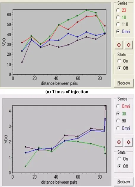
Next, the spatial variability in different direction is investigated, which is shown as figure 2. The first factor is times of injection as figure 2(a). It can be seen that the 110º series has the lowest variability at increasing separation distances. In the nearly orthogonal direction at 10º, variability increases much more rapidly.
(a) Times of injection
(c) Total injection
(d) Total oil production
Fig. 2: Spatial variability graph with different directions
The omnidirectional series is similar to an average in all directions and therefore it falls between the two series in this case. The 10º and 110º series reveal the extent of spatial variability with anisotropy and trending. The minimum spatial variability direction (110º) and the maximum (10º) implied the degree of spatial dependency across distance is greater in the north-east direction. Furthermore, in the west to east direction, especially at an approximate 110º direction, semi-variogram is somewhat similar. This implies the change of geological condition is very slowly. The second factor is injection pressure, which is shown as figure 2(b). It shows that all direction series has the lowest variability at increasing separation distances. We can guess the reason for this is that this factor is a production factor and not controlled by geological condition. Even though, it is still affected by geological condition. The third factor is total steam injection. The 10º and 100º series reveal the extent of spatial variability with anisotropy and trending. The minimum spatial variability direction (100º) and the maximum (10º) implied the degree of spatial dependency across distance is greater in the north-east direction. In direction 10º, variability increases very rapidly. In the nearly orthogonal direction at 100º, variability increases much slowly. The omnidirectional series is similar to an average in all directions and therefore it falls between the two series in this case.
The fourth factor is total oil production, which is shown as figure 2(d). It is similar with the second factor. It implies that total oil production is also a production factor. Overall, the first factor is similar with the third factor, and the second factor is similar with the forth. This reveals that steam injection times and total steam injection are controlled by geological condition. Injection pressure and total oil production are more affected by production rather than geological condition.
b. Risk images for all factors
shown as figure 3. In those maps, the risk is labeled from 0 to 255. 0 represents the minimum risk, and 255 represent the maximum risk. It can be found that the maximum risk factor is total steam rejection, and the minimum risk factor is total oil production.
(a) Times of injection
(b) Injection pressure
(c) Total injection
(d) Total oil production
Fig. 3: Risk assessment of each factor
c. OWA maps and risk analysis
[image:8.612.192.422.313.440.2]According to analytical hierarchy program (AHP) method, the relative importance between factors can be expressed by a significant value. The comparison matrix is constructed as table 1. Criterion weights are calculated, and the results are 0.0882, 0.1570, 0.2720, and 0.4828. According to the equation (5), order weights are also calculated. Order weights are 0.4, 0.3, 0.2, 0.1, and the risk assessment result is shown as figure 4.
Table 1 Comparison matrix
Total oil production
Injection pressure
Times of injection
Total injection Total oil production 1 1/2 1/3 1/5
Injection pressure 2 1 1/2 1/3
Times of injection 3 2 1 1/2
Total injection 5 3 2 1
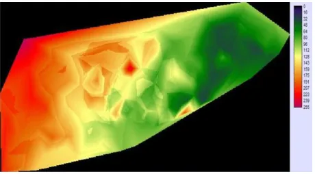
From figure 4, it is found that the risk of oil production increases gradually from southeast to northwest. The dangerous areas are located in the western, with risk values large than 120. Especially in the northwest part of the oilfield, values even more than 200. Therefore, more attention should be pain on those areas, and more comprehensive measures are needed to reduce the risk. In the eastern, values are properly less than 100, it reveal relatively safety areas.
Fig. 4: Result of risk assessment
Different variance images for different factors based on different sample data show greater uniformity in the variances across all areas. It is worth mentioning that the result of ordered weighted averaging method will equal to the result of weighted linear combination, if the order weights are 0.25, 0.25, 0.25, and 0.25 for the four influence factors. This means that weighted linear combination method is a special case of ordered weighted averaging method.
CONCLUSION
Most engineering data exhibit some spatial variability that can be described relative to distance and direction. Spatial variability present in the sample data is assessed in terms of distance and direction, and can be described as surfaces. During spatial variability analysis, it is necessary to spend a great deal of time modeling different directions with many different distances and lags, and confirming results with knowledge about the data distribution.
Acknowledgement
The author gratefully acknowledges the partial financial support for the work presented in this paper by the Sub-Topic of National Supporting Project of China (Grant NO.2009BAJ28B04-02B),China-Poland Inter-Governmental Science and Technology Cooperation Project (Grant NO. 2012-35-05), Science Foundation Project of Changzhou University (Grant NO. ZMF1102071), and Scholarship of Jiangsu Province (2013).
REFERENCES
[1]Scolozzi R., Geneletti D., 2011. Environ Manage, 47(3):368-83.
[2]Hu H.B., Liu H.Y., Hao J.F., etc., 2012. International Journal on Smart Sensing and Intelligent Systems, 5(4): 811-823.
[3]Taveau J., 2010. Journal of Loss Prevention in the Process Industries, 23:813-823. [4]Yager R.R., 2006. Information Sciences, 176:2933–2959.
[5]Yager R.R., 2008. Information Sciences, 178(1):363-380.