027
AN AUSM-BASED THIRD-ORDER COMPACT SCHEME FOR SOLVING
EULER EQUATIONS
M. A. H. Mohamad1, S. Basri1, I. Abd. Rahim2 and M. Mohamad3
1Dept. of Aerospace Engineering, Faculty of Engineering, University Putra Malaysia, Selangor, Malaysia.
2Dept. of Plant & Automotive Engineering, Faculty of Mechanical & Manufacturing Engineering,
University College of Technology Tun Hussein Onn, Johor, Malaysia.
3Dept. of Mathematics, Science Studies Centre, University College of Technology Tun Hussein Onn,
Johor, Malaysia.
E-mail: [email protected]
ABSTRACT
In this paper, a third-order compact upwind scheme is given for calculating flows containing discontinuities. The scheme utilizes the AUSM flux splitting method and a third-order compact upwind space discretization relation for calculating third-order numerical flux function. TVD shock capturing properties of the scheme are achieved through a minmod flux limiter. A multistage TVD Runge-Kutta method is employed for the time integration. Computations are performed for two typical one-dimensional problems containing shocks, namely, the steady flow in a divergent nozzle and the unsteady shock tube problem. First-order and third-order numerical results are presented in comparison with the exact solutions. Computed results with KFVS method are also presented.
Key words: Third-Order Compact Upwind Scheme, AUSM scheme, KFVS scheme
INTRODUCTION
High-order compact schemes have attracted much attention in recent years due to their narrow grid stencil and a possible enhanced accuracy over the non-compact schemes [1]. Different approaches for high-order compact spatial discretization have been proposed during the last 25 years.
Lele [1] has presented and analyzed a class of high-order central schemes and introduced the notion of resolution efficiency. Central compact schemes have been used for solving inviscid flows [2] and viscous flows [3,4,5]. However, numerical instabilities and spurious oscillations are often encountered in the solution of convection-dominated flows. These instabilities can be suppressed either by adding high-order dissipation terms [2] or by using filtering [4].
Shock discontinuities give rise to high frequency oscillations even in smooth regions of the flow due to odd-even decoupling. Therefore, excessive smoothing is required to capture strong shocks. This in turn will considerably degrade the solution scheme. Consequently, central schemes are not robust enough for flows with discontinuities. On the other hand, upwind schemes are expected to be more robust and to yield superior results. Cockburn and Shu [6], using the idea of TVD (total variation diminishing) with a modified flux limiter, have formulated a family of nonlinear stable compact schemes for nonlinear scalar conservation laws. Upwinding is introduced through Lax-Friedrichs flux-splitting method.
Deng and Maekawa [7] have presented higher-order nonlinear schemes for capturing discontinuities. They used Roe’s approximate Riemann solver and a fourth-order cell-centered compact scheme to calculate higher-order numerical flux at a cell interface. The left and right states are computed through compact adaptive interpolation in the spirit of ENO [8] reconstruction. The drawback of Roe’s approximate Riemann solver and ENO schemes is that they are computationally uneconomical. Ravichandran [9] has developed a third-order flux-splitting variant TVD upwind scheme. Only steady state results are reported.
for capturing of intense shocks and rarefaction waves. However, while FVS is based on scalar calculations and FDS is based on matrix calculations.
The high-order compact schemes developed by Cockburn and Shu [6], Mawlood et al. [14], and Ravichandran
[9] among others are examples of FVS schemes. The drawback of FVS methods is that they have accuracy problems in resolving shear layer regions due to the excessive numerical dissipation error associated with them.
Liou and Steffen [15] have proposed AUSM (Advection Upstream Splitting Method) that has the accuracy of FDS schemes and the robustness and efficiency of FVS schemes. In this method, the inviscid flux at a cell interface is split into a convective contribution, upwinded in the direction of the flow and a pressure contribution which is upwinded based on acoustic considerations. The direction of the flow is determined by the sign of a Mach number defined by combining information from both the left and right states about the cell interface.
The main purpose of the present work is to develop a high-order compact shock capturing scheme based on AUSM flux splitting method. A third-order, upwind-based compact scheme proposed by Zhong [16] is used to obtain the higher-order numerical fluxes. TVD shock capturing properties are obtained through the minmod flux limiters presented by Cockburn and Shu [6] and Ravichandran [9]. The scheme is tested with two typical one dimensional problems containing shocks. The first problem is a steady supersonic-subsonic flow in a divergent nozzle and the second is a time dependent shock tube problem. First-order and third-order results are presented in comparison with the exact solutions. Results using the KFVS method [13] are also presented.
THE BASIC DISCRETIZATION METHOD
Spatial Discretization and Numerical Fluxes
The model equation for nonlinear scalar conservation law in one-dimensional space can be written as [10,11]
0
)
(
=
∂
∂
+
∂
∂
x
u
f
t
u
(1)
with the subject to the given initial condition [10,11]
u
(
x
,
0
)
=
u
0(
x
)
(2)where
x
u
f
∂
∂
(
)
is some vector-valued function of u. Equation (2), is specialised to
)
0
(
)
0
,
(
)
0
(
)
0
,
(
>
≡
<
≡
x
u
x
u
x
u
x
u
R L
(3)
Equation (1) can be written in split flux form as [9]
0
)
(
)
(
=
∂
∂
+
∂
∂
+
∂
∂
+ −x
u
f
x
u
f
t
u
(4)
where
f
(
u
)
=
f
+(
u
)
+
f
−(
u
).
This flux vector splitting has been introduced by [11]. The split fluxes)
(
u
f
+ andf
−(
u
)
are also homogeneous functions of degree one in u [18]. Conservative semidiscretization ofequation (4) can be written as [9]
0
/
)
ˆ
ˆ
(
1/2−
1/2∆
=
+
∂
∂
−
+
f
x
f
t
u
i i
where
f
ˆ
i+1/2 andf
ˆ
i−1/2 is known as the numerical flux function. First-order upwind approximation to the numerical flux is given by [9]− + − − − + + +
−
=
+
=
i i i i i if
f
f
f
f
f
1 2 / 1 1 2 / 1ˆ
ˆ
(6)Following Ravichandran [9], a high-order numerical flux can be obtained as follows. The numerical flux
2 / 1
ˆ
+ if
is decomposed into positive and negative parts,f
ˆ
i++1/2 andf
ˆ
i−+1/2 such that− + +
+
+1/2
=
ˆ
1/2+
ˆ
1/2ˆ
i i
i
f
f
f
(7)The decomposed numerical fluxes are defined such that
m m m 2 / 1 2 / 1
ˆ
ˆ
− +−
=
i ii
f
f
F
(8)where
F
im/
∆
x
is a high-order approximation to the derivativex
u
f
i∂
∂
m(
)
, to be determined by a high-order
compact scheme.
Zhong [16] has presented a third-order approximation to a first derivative by an upwind based compact relation as m m m m m m m
m
m
m
1 1
1
1
60
15
52
.
5
15
37
.
5
75
.
18
F
i±+
F
i+
F
i=
±
f
i±f
if
i (9)Equation (6) can be written for the interior points
i
=
2
toi
=
N
−
1
. For the boundary pointsi
=
1
and
i
=
N
, the following second order explicit relations are used
F
1m=
−
1
.
5
f
1m+
2
f
2m−
0
.
5
f
3m (10)F
Nm=
1
.
5
f
Nm−
2
f
Nm−1+
0
.
5
f
Nm−2 (11)
Plugging equation (8) in equation (9) yields the following relations for the interior points
i
=
2
toi
=
N
−
1
.+ + + + + + + +
−
+
i+
i=
i+
ii
f
f
f
f
f
ˆ
60
ˆ
11
.
25
ˆ
37
.
5
52
.
5
75
.
18
1/2 1/2 3/2 1 (12)− − + − + − + −
−
+
i+
i=
i+
ii
f
f
f
f
f
ˆ
60
ˆ
18
.
75
ˆ
52
.
5
37
.
5
25
.
11
1/2 1/2 3/2 1 (13)With
F
1m andF
Nm evaluated explicitly, two sets of (N - 1) equations are to be inverted for the split numericalfluxes
f
ˆ
im+1/2. Before using these fluxes it is necessary to limit their values and this is achieved by defining theand limiting by the limiter
)
,
ˆ
mod(
min
ˆ
)
,
ˆ
mod(
min
ˆ
2 / 1 ) ( 2 / 1 2 / 1 ) ( 2 / 1 − − + − + + + + + +=
=
D
f
d
f
d
D
f
d
f
d
i m i i m i (15)The third-order TVD flux differences of [17] may be used here
(min
mod(
,
)
2
min
mod(
,
))
6
1
1
1 + + + + + +−
+ − + +
=
+
i i ii
f
f
f
f
D
δ
λδ
δ
λδ
(16)
(min
mod(
,
)
2
min
mod(
,
))
6
1
1 1 − + + − + − + − + + −=
+
i i ii
f
f
f
f
D
δ
λδ
δ
λδ
(17)where
1
≤
λ
≤
4
.The limited numerical fluxes are then calculated from
) ( 2 / 1 1 ) ( 2 / 1 ) ( 2 / 1 ) ( 2 / 1
ˆ
ˆ
ˆ
ˆ
m i i m i m i i m if
d
f
f
f
d
f
f
− + − + − + + + + + +−
=
+
=
(18) and
f
ˆ
i+(m1/)2=
f
ˆ
i++1(m/2)+
f
ˆ
i−+1(/m2) (19)The min mod function can be defined as
<
>
<
>
<
=
0
)
(
0
0
)
(
,
0
)
(
,
)
,
mod(
min
ab
if
ab
a
b
if
b
ab
b
a
if
a
b
a
(20)EULER EQUATIONS AND FLUX SPLITTING SCHEME
The one-dimensional Euler equation may be written as
=
0
∂
∂
+
∂
∂
x
E
t
Q
(21) where,
=
e
u
Q
ρ
ρ
ρ
+
=
uH
p
u
u
E
ρ
ρ
ρ
2and ρ, u, p, e and H are the density, velocity, pressure, total energy, and total enthalpy respectively. The total
ρ
p
e
H
=
+
(22)and for a perfect gas
2
2
1
)
1
(
u
p
e
+
−
=
γ
ρ
(23)where
γ
is the ratio of specific heat and takes the value of 1.4 for air.The extension of the scalar high order numerical fluxes developed above to Euler equations is straightforward.
The AUSM flux splitting technique used here is detailed in references [15,16]. Once the split fluxes
E
i±areobtained then the method described above is used to obtain the higher order numerical fluxes. Equation (18) is, thus, written in a semidiscretized form as
L
(
Q
)
t
Q
=
∂
∂
(24)
where
x
E
E
Q
L
m i m
i
−
∆
−
=
(
+ −)
/
)
(
) (
2 / 1 ^ ) (
2 / 1 ^
(25)
Using the method-of-lines [9], the systems of equations (21) are integrated by a multistage TVD Runge-Kutta scheme [17].
BOUNDARY CONDITIONS
For the supersonic-subsonic nozzle problem considered in this paper, one type of boundary conditions i.e. inflow/outflow is encountered. At the supersonic inflow, values of velocity, density and pressure are specified while at the subsonic outflow the velocity is specified and the density and pressure are extrapolated from the interior. For the shock tube problem, a short time span for unsteady flow is considered such that the waves will not reach the end walls and so conditions at these boundaries are held fixed.
RESULTS AND DISCUSSIONS
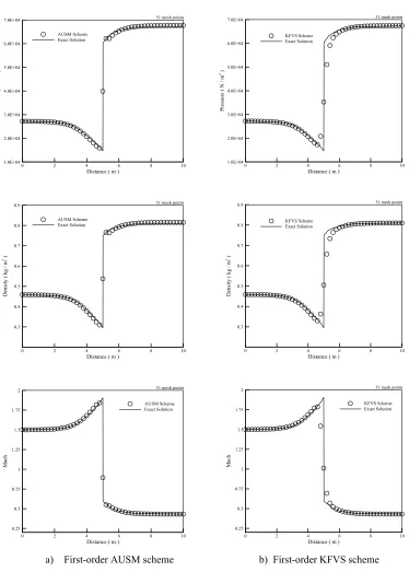
In this study, two problems are considered as test cases for the developed scheme. Results are presented for both the AUSM and the KFVS variants of the scheme. Results are also shown with first-order accurate upwind space discretization. The first problem considered is a quasi one-dimensional supersonic-subsonic flow in a divergent
nozzle. The nozzle cross-section S(x) varies according to
S(x) = 1.398 + 0.347 tanh
(
0
.
8
(
x
−
4
)
)
; 0 ≤x≤ 10 The inflow and outflow conditions are(ρ1, u1, p1) = (0.459, 432.5, 0.2724 x 10⁵)
(ρN, uN, pN) = (0.811, 146.94, 0.673 x 10⁵)
These conditions correspond to a normal shock at x = 5 with supersonic flow at the inlet Mach number M1 = 1.5
and subsonic flow at the outlet Mach number MN = 0.431. Calculation are performed with a time step, ∆t
corresponding to Courant-Friedrichs-Lewy, CFL number = 1. The number of points used to solve this problem is N = 51. The integration in time is continued until steady state is reached. The solution is assumed to converge
when the absolute value of the residual in pressure pn+1– pn≤ 0.1.
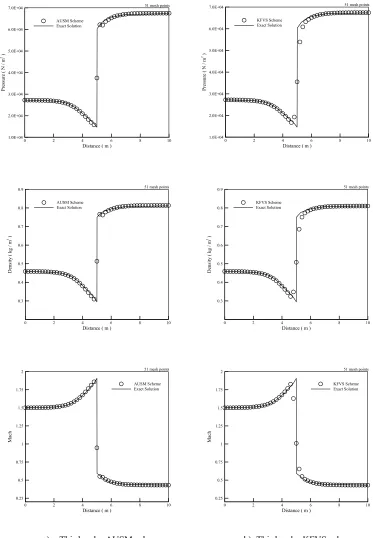
false diffusion of first-order upwinding, is evident with both flux splitting methods. In Fig. 2 results obtained by the third-order schemes are shown. The shock capturing properties of the AUSM are improved while the KFVS method produces oscillatory solution behind the shock.
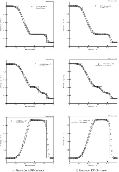
The second problem considered is the unsteady shock tube problem. This problem is an interesting test case to assess the ability of a compressible code to capture shocks and contact discontinuities and to produce exact
profiles in the rarefaction wave. The problem spatial domain is 0 ≤x ≤ 1. The initial solution of the problem
consists of two uniform states, termed as left and right states, separated by a discontinuity at x = 5. As in the first
problem, results are obtained using first-order and third-order upwind schemes with both the AUSM and the KFVS methods. The number of mesh points used is 101 and CFL = 0.2. The initial conditions of the left and right states are
(ρL, uL, pL) = (1, 0, 1)
(ρR, uR, pR) = (0.125, 0, 0.1)
The wave pattern of this problem consists of a rightward moving shock wave, a leftward moving rarefaction wave and a contact discontinuity separating the shock and rarefaction waves and moving rightward. Fig. 3 shows results obtained by the first order accurate schemes for the distribution of pressure, density and velocity
along the tube at time, t = 0.2 units, in comparison with the exact solution. Although the solution contains no
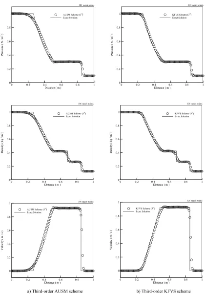
oscillations the smearing of all types of discontinuities is quite clear. In Fig. 4 the third-order results are shown. The improvement in resolving the different types of discontinuities is clear. The shock discontinuity is resolved more accurately by the AUSM scheme as can be seen from the velocity plot. The contact discontinuity is resolved equally by both schemes; however, a small jump is observed ahead of the contact discontinuity in the result of the AUSM scheme as can be seen in the density and velocity plots. The calculated profiles of all variables in the rarefaction wave agree very well with the exact solution. The KFVS variant shows slightly
Distance ( m )
Pr
es
su
re
(
N
/m
2)
0 2 4 6 8 10
1.0E+04 2.0E+04 3.0E+04 4.0E+04 5.0E+04 6.0E+04 7.0E+04
AUSM Scheme Exact Solution
51 mesh points
Distance ( m )
Pre
ssure
(
N
/m
2)
0 2 4 6 8 10
1.0E+04 2.0E+04 3.0E+04 4.0E+04 5.0E+04 6.0E+04 7.0E+04
KFVS Scheme Exact Solution
51 mesh points
Distance ( m )
Dens
ity
(
kg
/m
3)
0 2 4 6 8 10
0.3 0.4 0.5 0.6 0.7 0.8 0.9
AUSM Scheme Exact Solution
51 mesh points
Distance ( m )
Den
sity
(
kg
/m
3)
0 2 4 6 8 10
0.3 0.4 0.5 0.6 0.7 0.8 0.9
KFVS Scheme Exact Solution
51 mesh points
Distance ( m )
Mach
0 2 4 6 8 10
0.25 0.5 0.75 1 1.25 1.5 1.75 2
AUSM Scheme Exact Solution
51 mesh points
Distance ( m )
Mach
0 2 4 6 8 10
0.25 0.5 0.75 1 1.25 1.5 1.75 2
KFVS Scheme Exact Solution
51 mesh points
[image:7.612.115.489.155.678.2]a) First-order AUSM scheme b) First-order KFVS scheme
Distance ( m )
Pre
ssu
re
(
N
/m
2)
0 2 4 6 8 10
1.0E+04 2.0E+04 3.0E+04 4.0E+04 5.0E+04 6.0E+04 7.0E+04
AUSM Scheme Exact Solution
51 mesh points
Distance ( m )
Pre
ssure
(
N
/m
2)
0 2 4 6 8 10
1.0E+04 2.0E+04 3.0E+04 4.0E+04 5.0E+04 6.0E+04 7.0E+04
KFVS Scheme Exact Solution
51 mesh points
Distance ( m )
D
ens
ity
(
kg
/m
3)
0 2 4 6 8 10
0.3 0.4 0.5 0.6 0.7 0.8 0.9
AUSM Scheme Exact Solution
51 mesh points
Distance ( m )
D
ens
ity
(
kg
/m
3)
0 2 4 6 8 10
0.3 0.4 0.5 0.6 0.7 0.8 0.9
KFVS Scheme Exact Solution
51 mesh points
Distance ( m )
M
ach
0 2 4 6 8 10
0.25 0.5 0.75 1 1.25 1.5 1.75 2
AUSM Scheme Exact Solution
51 mesh points
Distance ( m )
M
ach
0 2 4 6 8 10
0.25 0.5 0.75 1 1.25 1.5 1.75 2
KFVS Scheme Exact Solution
51 mesh points
[image:8.612.112.485.106.644.2]a) Third-order AUSM scheme b) Third-order KFVS scheme
Distance ( m )
P
ressu
re
(
N
/m
2)
0 0.2 0.4 0.6 0.8 1
0 0.2 0.4 0.6 0.8
1 AUSM Scheme (1st)
Exact Solution 101 mesh points
Distance ( m )
Pr
es
su
re
(
N
/m
2)
0 0.2 0.4 0.6 0.8 1
0 0.2 0.4 0.6 0.8
1 KFVS Scheme (1st)
Exact Solution 101 mesh points
Distance ( m )
D
en
sity
(
kg
/m
3)
0 0.2 0.4 0.6 0.8 1
0 0.2 0.4 0.6 0.8
1 AUSM Scheme (1st)
Exact Solution 101 mesh points
Distance ( m )
D
en
sity
(
kg
/m
3)
0 0.2 0.4 0.6 0.8 1
0 0.2 0.4 0.6 0.8
1 KFVS Scheme (1st)
Exact Solution 101 mesh points
Distance ( m )
V
elo
ci
ty
(
m
/s
)
0 0.2 0.4 0.6 0.8 1
0 0.2 0.4 0.6 0.8 1
AUSM Scheme (1st ) Exact Solution
101 mesh points
Distance ( m )
V
elo
city
(
m
/s
)
0 0.2 0.4 0.6 0.8 1
0 0.2 0.4 0.6 0.8 1
KFVS Scheme (1st) Exact Solution
101 mesh points
[image:9.612.111.529.81.685.2]a) First-order AUSM scheme b) First-order KFVS scheme
Distance ( m )
Pre
ssur
e
(
N
/m
2)
0 0.2 0.4 0.6 0.8 1
0 0.2 0.4 0.6 0.8
1 AUSM Scheme (3rd)
Exact Solution
101 mesh points
Distance ( m )
Pre
ssur
e
(
N
/m
2)
0 0.2 0.4 0.6 0.8 1
0 0.2 0.4 0.6 0.8
1 KFVS Scheme (3rd)
Exact Solution
101 mesh points
Distance ( m )
D
en
sity
(
kg
/m
3)
0 0.2 0.4 0.6 0.8 1
0 0.2 0.4 0.6 0.8
1 AUSM Scheme (3rd
) Exact Solution
101 mesh points
Distance ( m )
D
en
sity
(
kg
/m
3)
0 0.2 0.4 0.6 0.8 1
0 0.2 0.4 0.6 0.8
1 KFVS Scheme (3rd
) Exact Solution
101 mesh points
Distance ( m )
V
elo
city
(
m
/s
)
0 0.2 0.4 0.6 0.8 1
0 0.2 0.4 0.6 0.8 1
AUSM Scheme (3rd) Exact Solution
101 mesh points
Distance ( m )
Vel
oci
ty
(
m
/s
)
0 0.2 0.4 0.6 0.8 1
0 0.2 0.4 0.6 0.8 1
KFVS Scheme (3rd) Exact Solution
101 mesh points
[image:10.612.106.526.82.684.2]a) Third-order AUSM scheme b) Third-order KFVS scheme
CONCLUSIONS
A third-order accurate TVD compact shock-capturing scheme is developed using the AUSM flux splitting method. The scheme is tested by performing calculations for a quasi one-dimensional supersonic-subsonic nozzle flow and a shock tube problem. Results are also presented with a scheme based on KFVS. The KFVS variant has shown oscillations behind the stationary shock wave in the nozzle flow problem. However, the KFVS variant is found to capture contact and rarefaction discontinuities in the shock tube problem more accurately than the AUSM variant.
REFERENCES
1. Lele, S. K. (1992) Compact Finite Difference Schemes with Spectral-Like Resolution. Journal of
Computational Physics, 103:16-42.
2. Ekaterinaris, J. A. (1999) Implicit High–Resolution, Compact Schemes for Gas Dynamics and
Aeroacoustics. Journal of Computational Physics, 156: 272-299.
3. Ekaterinaris, J. A. (2000) Implicit High-Order Accurate In-Space Algorithms for The Navier Stokes
Equations. AIAA Journal, 38:1591-1602.
4. Visbal, M. R. and Gaitonde, P. V. (1999) High Order-Accurate Methods for Complex Unsteady Subsonic Flows. AIAA Journal, 10: 358-366.
5. Mawlood, M. K., Asrar, W., Basri, S. and Ahmad, M. H. M. (2001) High-Order Compact Finite
Difference Solution of Navier-Stoke Equations. Jurnal Mekanikal, (12): 83-95.
6. Cockburn, B. and Shu, C. W. (1994) Nonlinearly Stable Compact Schemes for Shock Calculation.
SIAM Journal on Numerical Analysis, 31(3): 607-627.
7. Deng, X. and Maekawa, H. (1997) Compact High–Order Accurate Nonlinear Schemes. Journal of
Computational Physics, 130: 77-91.
8. Harten, A., Engquist, B., Osher, S. and Chakravarthy, S. (1987) Uniformly High Order Accurate
Essentially Non-Oscillatory Schemes, III. Journal of Computational Physics, 71: 231-303.
9. Ravichandran, K. S. (1997) High Order KFVS Algorithms Using Compact Upwind Difference
Operators. Journal of Computational Physics, 130: 161-173.
10. Roe, P. L. (1981) Approximate Riemann Solvers, Parameter Vectors, and Difference Schemes. Journal
of Computational Physics, 43: 357-372.
11. Steger, J. L. and Warming, R. F. (1981) Flux Vector Splitting of the Inviscid Gas Dynamic Equations
with Application to Finite Difference Methods. Journal of Computational Physics, 40: 263-293.
12. Van Leer, B. (1982) Flux Vector Splitting for the Euler Equation. Lecture Notes in Physics, 170:
507-512.
13. Deshpande, S. M. and Kulkarni, P. S. (1998) New Developments in Kinetic Schemes. Computers Math.
Application, 35(112): 75-93.
14. Mawlood, M. K., Asrar, W., Omar, A.A. and Basri, S. (2003) A High-Resolution Compact Upwind
Algorithm for Inviscid Flows. 41st Aerospace Sciences Meeting and Exhibit Conference, AIAA
2003-0076, USA.
15. Liou, M. S. and Steffen, C. J. Jr. (1993) A New Flux Splitting Scheme. Journal of Computational
Physics, 107: 23-39.
16. Zhong, X. (1998) High-Order Finite-Difference Schemes for Numerical Simulation of Hypersonic
Boundary-Layer Transition. Journal of Computational Physics, 144: 662-709.
17. Yee, H. C. (1987) Upwind and Symmetric Shock Capturing Schemes. NASA TM 89464.
18. Hirsch, C. (1990) Numerical Computation of Internal and External Flows. Vol. 2: Computational
Methods for Inviscid and Viscous Flows. John Wiley and Sons, UK.
ABBREVIATIONS
AUSM Advection upstream splitting method
CFL Courant-Friedrichs-Lewy number
ENO Essentially non-oscillatory schemes
FDS Flux-difference splitting
FVS Flux-vector splitting
KFVS Kinetic flux-vector splitting
NOTATIONS
b
a
,
Coefficients in high-order compact schemesf
d
ˆ
Flux differenceD
Diffusion numberE
Flux vectorse
Total energyi
F
High-order approximation to first derivativeF
Flux vectorsf
Scalar fluxf
ˆ
Flux functionH
Total enthalpyi
Inner layerL
Characteristic lengthM
Mach numberN
Maximum number of grid pointsp
PressureQ
Conservative variable vectoru
Velocity componentsλ
Eigenvalue+
δ
Forward difference operators∆
Increment in time and spaceγ
Specific heat ratio, for air = 1.4ρ
DensitySuperscripts
n n-th time level
m Modified (limited) flux
Subscripts
l, N Inflow and outflow condition