Statistical Hough Transform

Short Papers

Statistical Hough Transform

Rozenn Dahyot

Abstract—The Standard Hough Transform is a popular method in image processing and is traditionally estimated using histograms. Densities modeled with histograms in high dimensional space and/or with few observations, can be very sparse and highly demanding in memory. In this paper, we propose first to extend the formulation to continuous kernel estimates. Second, when dependencies in between variables are well taken into account, the estimated density is also robust to noise and insensitive to the choice of the origin of the spatial coordinates. Finally, our new statistical framework is unsupervised (all needed parameters are automatically estimated) and flexible (priors can easily be attached to the observations). We show experimentally that our new modeling encodes better the alignment content of images.

Index Terms—Hough transform, Radon transform, kernel probability density function, uncertainty, line detection.

Ç

1

I

CONSIDERINGa set of points in a 2D plane, the Hough transform maps each point of coordinatesðx; yÞto all the variablesð; Þin the Hough space with the relation:

¼x cosþy sin: ð1Þ

If a set of observations Sxy¼ fðxi; yiÞgi¼1N is aligned on one straight line with coefficients ð_;^_{Þ^, then the family of curves}

Cið; Þ: ¼xi cosþyi sin;8i2 ½1;N

f g intersects in the

Hough space at ð_;^_{Þ^. This property is used to robustly perform} the estimation ofð;^^Þby incrementing a discrete two-dimensional histogram defined on the space of variablesð; Þfor each point of the curvesfCig. The highest bin of this histogram allows then to estimate the parametersð;^^Þof the line. This technique has been proposed to recover lines in images more than four decades ago [1] and refined (as expressed here) in the early 1970s [2]. Many works have since been proposed both to generalize the Hough transform to more complex shapes than straight lines and to improve its computational efficiency [3]. The Hough transform has recently been proven to be a statistically robust estimator for finding lines [4]. The Hough transform has, however, one main weakness: the probability density functionpð; Þof the parametersð; Þin the Hough space is estimated using a discrete two-dimensional histogram [5]. Therefore, the trade-off in between the number of bins in the histogram and the number of available observations is crucial. Too many bins for too few observations would lead to a sparse representation of the density. Too few bins would also reduce the resolution in the Hough space, and therefore, limit the precision of the estimates. Hence, it is important to extract the most relevant information from all available observations to model the distribution ofð; Þ. To overcome histogram limitations, the

main contribution of this paper is to propose a statistical kernel modeling of the Hough transform so that the resulting estimate ^

pð; Þ is continuous and includes as much information as available. The variablesx; y; ; andare modeled as continuous random variables from which some observations may (or may not) be available. In particular, we define the following sets of observations:

. Sxy¼ fðxi; yiÞgi¼1Nis the set of observations of the spatial random variablesðx; yÞ. This set is used in the Standard Hough Transform.

. Sxy¼ fði; xi; yiÞgi¼1N is the set of the location with an observation of the angle . Indeed, when considering images, the angle of the gradient can locally be computed and used as an observation of.

. S¼ fði; iÞgi¼1N: knowingi,xi, andyi, the measurei can be computed using (1) and also used as an observation. In addition to the observations, we attached a prior pi to each observationi. Our statistical framework completely generalizes the Standard Hough Transform and shows the clear links between the Hough and the Radon transforms. The second main contribution of this paper is to take advantage of the relation (1) between the random variables. This allows us to propose three different estimates of pð; Þ for each set of observations (Sxy, Sxy, and S). This new framework is presented in Section 3.

One drawback of kernel modeling is that it requires the estimation of bandwidths. We propose in Section 4 a method to set automatically those bandwidths. We show in Section 5 how accurate and also how resistant to noise our estimates are. Many articles have been published on the Hough transform in the last 50 years or so and it has been applied to many different applications, such as image and video [6] processing, astronomy [7], or geoscience [8]. We start with a nonexhaustive review in Section 2 on local appearance-based features and the Hough Transform.

2

C

2.1 Distribution of Local Appearance-Based Measures

Schmid et al. [9] have defined local descriptors of the intensity surface of images to detect interesting points (e.g., corners) and match images. Using similar local appearance-based features, Schiele and Crowley [10] have proposed to model their distribu-tions using multidimensional histograms, and detection and recognition of objects can then be performed by comparing histograms. More recently, due to the increasing computational power of computers, kernel modeling [11] succeeded histograms for the modeling of the distribution of local descriptors and the Mean-shift procedure, used for finding modes of kernel densities, has found many applications in computer vision [12].

2.2 Local Hough Features

We note ðx; yÞ !Iðx; yÞ a surface image and its first order derivatives Ixðx; yÞ and Iyðx; yÞ. For each pixel i at location ðxi; yiÞ, the following three local appearance-based measures are computed in [13]:

krIik ¼ krIðxi; yiÞk ¼

ffiffiffiffiffiffiffiffiffiffiffiffiffiffiffiffiffiffiffiffiffiffiffiffiffiffiffiffiffiffiffiffiffiffiffiffiffiffiffiffiffiffiffi I2

xðxi; yiÞ þIy2ðxi; yiÞ

q

i¼ðxi; yiÞ ¼arctan

Iyðxi; yiÞ Ixðxi; yiÞ

i¼ðxi; yiÞ ¼xi

Ixðxi; yiÞ krIðxi; yiÞkþ

yi

Iyðxi; yiÞ krIðxi; yiÞk

: 8

> > > > > > < > > > > > > :

ð2Þ . The author is with the Department of Statistics, School of Computer

Science and Statistics, Trinity College Dublin, Room 128, Lloyd Institute, Dublin 2, Ireland. E-mail: [email protected].

Manuscript received 25 Mar. 2008; revised 14 Oct. 2008; accepted 20 Nov. 2008; published online 26 Nov. 2008.

Recommended for acceptance by M. Lindenbaum.

For information on obtaining reprints of this article, please send e-mail to: [email protected], and reference IEEECS Log Number

TPAMI-2008-03-0162.

No edge segmentation is performed in [13]: The observations of all three measuresfði; i;krIikÞgi¼1;;Nare computed for all pixels in the image and the joint distributionpkrIkð; ;krIkÞis estimated

by a three-dimensional histogram. The estimated density is then used to detect appearing, disappearing, or changing objects in a sequence [13].

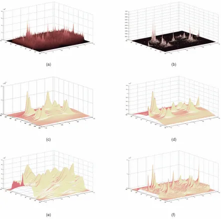
Integrating this 3D histogram w.r.t. the magnitude of the gradient gives an estimate (2D histogram) of the density function pð; Þthat is noisy (all pixels in the image have been used). An example of such histogram computed for the image in Fig. 3b is shown in Fig. 1a.

In another approach proposed by Ji and Haralick [14], the imageIðx; yÞis locally approximated by a plane:

Iðx; yÞ ¼yþxþþ; ð3Þ

where is a centered Gaussian noise. An estimate of the Hough parameters is then computed by

tani¼ ^ ^

i¼xicosiþyisini;

8 > < >

: ð4Þ

where ^ and^are locally estimated using least squares on the neighborhood ofðxi; yiÞ. The spatial derivatives ofIðx; yÞmodeled in (3) give also estimates forand[14]. The standard errori made in computing the angleican also be quantified by [14], [15]:

2 i¼

2 krIik2

; ð5Þ

where2 _{is the variance of the noise on the derivativesI} xandIy, which can be known in advance or estimated from the observa-tions of the magnitude of the gradient [16], [17], [18]. The variance in (5) confirms the intuition that the uncertainty of the computed orientation i increases as the gradient magnitude decreases. A similar result has also been found in [19].

For the observationi, an estimate of its variance can also be computed for pixeli:

Fig. 1. Statistical Hough transform on the imagediamondin Fig. 3b with additional Gaussian noise N ð0;202_{Þ. (a) Histogramhð; Þ(P1). (b) Weighted histogram}

2

i¼cos

2

i2xiþsin

2 i2yiþ

2

iðyicosixisiniÞ

2_{; ð6Þ}

where 2 xi and

2

yi are the variances of the spatial coordinates

ðxi; yiÞ. As noted in [14], the origin of the spatial coordinates is better chosen in the center of the image in order to limit the error done on the featureisince its variance (c.f., (6)) depends on the locationðxi; yiÞ.

For each observationði; iÞfor the pixeliat locationðxi; yiÞ, we can compute their uncertaintyði; iÞusing (5) and (6), once the spatial uncertaintyxiandyiare set (see Section 4.2). A weighted histogram can then be computed using 1

2 ii as weights [14]. It is shown in Fig. 1b. The localization of the peaks are much easier to detect than in Fig. 1a, but it is still a discontinuous representation of the densitypð; Þ.

2.3 Recent Works on the Hough Transform

Many works have been published on the Hough Transform since its first publication [1]. Recently, Aggarwal and Karl proposed to robustly detect lines in noisy environment in the Hough space by adding prior modeling on the variables ð; Þ [20]. Several probabilistic Hough transforms, related to the RANSAC approach [21], have also been proposed [22], [23]. Of particular interest for this paper is the Meanshift clustering approach in the Hough domain proposed by Bandera et al. [23], where a continuous kernel modeling of pð; Þ with variable bandwidth is introduced. However, their modeling is deduced from a very different approach and their resulting process requires many parameters to be manually tuned.

In [24], a probabilistic interpretation of the Hough transform is proposed: The histogram Hð; Þ of the variables ð; Þ in the standard Hough transform is interpreted as logðpð; jSxyÞÞ /

PN

i¼1logpð; jðxi; yiÞÞ. In [6], the standard Hough transform is extended and related to a robust M-estimator function [25].

Usually histograms are interpreted as being direct estimates of a probability density function [11] and not their logarithm. We propose in Section 3 another statistical interpretation of the Hough transform.

2.4 Reliability, Confidence, and Uncertainty

of Local Features

The notion of uncertainty of a measurement is the amount by which an observed value differs from its true value. For instance, Steele and Jaynes [26] studied the uncertainty of the spatial localization of a corner detector. The notion of repeatability of a detector [9], defined by its robustness at detecting image features independently from perturbations in the imaging conditions, is closely related to uncertainty. A measurement with high uncertainty under a particular perturbation is indeed unlikely to be repeatable.

Another way to understand uncertainty is in considering that an observation is a random sample from an unknown distribution. For instance, lets assume a Gaussian distribution of the angle centered on its estimateiand with standard deviation as defined in (5). Now, if we consider two instances of the same scenedðx; yÞ, I1ðx; yÞ ¼dðx; yÞ þð1Þ_{ðx; yÞ and I2ðx; yÞ ¼dðx; yÞ þ}ð2Þ_{ðx; yÞ, with}

Gaussian noise N ð0; 2_{Þ, then the measurements of the angle} in flat areas (i.e., when the gradient is close to zero) are going to be randomly sampled from a uniform distribution on the interval ½ =2; =2. Therefore, it is unlikely that the measurements ofon flat areas are corresponding in both images at the same position ðx; yÞ. The measure of the angle is not a reliable measurement to match images when it has been computed on uniform regions. On the contrary, when there is a contour (dx6¼0 or dy6¼0), the variance of the measureis small. As a consequence, the observed angle is sampled from a narrow Gaussian distribution and it

should accurately repeat itself from one instance of an imageI1to anotherI2.

One traditional way to deal with this uncertainty on the features is to throw away unreliable observations before inferring decision. For instance, in the Standard Hough Transform, only pixels on the edges are used (i.e., pixels i with high gradient magnitude, and therefore, low uncertainty on the anglei). Edge selection can be risky as relevant information can be lost in the process. In the next sections, we propose a new formalism that does not require edge segmentation as a preliminary step.

3

S

H

T

From the sets of observationsS,Sxy, andSxy, we propose three estimates of the probability density functionpð; Þusing kernel modeling [11].

3.1 Kernel Density Modeling ofp^ð; jSÞ

Using the set of observations S, we model the distribution pð; jSÞusing kernels by

^ p ; jS ¼X N

i¼1 1 hi

k i

hi

1 hi

k i

hi

pi; ð7Þ

wherehi andhi are the variable bandwidths. Their estimations are explained in Section 4. The kernelskðÞandkðÞ have been chosen Gaussians so that (7) gives a continuous and smooth estimate of the densitypð; Þ.

3.2 Kernel Density Modeling ofp^ð; jSxyÞ

In the previous section, we have used a subset of the observations leaving apart the locationfðxi; yiÞgi¼1N. We want now to take into account those observations to model first the densitypxyð; ; x; yÞ. Using the Bayes formula, we can write

pxyð; ; x; yÞ ¼pjxyðj; x; yÞpxyð; x; yÞ: ð8Þ

As noticed by Bonci et al. [15], whenx; y; are known, the variable is deterministic, by definition, in (1). Therefore, we propose to model the conditional probability as follows:

pjxyðj; x; yÞ ¼ðxcosysinÞ; ð9Þ

where ðÞ is the Dirac distribution. As a consequence, only pxyð; x; yÞ is to estimate using kernels with the set of observatons Sxy:

^

pxyð; x; yjSxyÞ ¼

XN

i¼1 ^

pxyð; x; yji; xi; yiÞpi

¼X

N

i¼1 ^

pðjiÞp^xðxjxiÞp^yðyjyiÞpi

¼X

N

i¼1 1 hxi

kx xxi

hxi

₁

hyi

ky yyi

hyi

1

hi

k i

hi

pi:

ð10Þ

Note that we have assumed the variables,x, andyindependent given their observationsði; xi; yiÞ. By integration with respect to the spatial variables ðx; yÞ, an estimate of the Hough transform pð; Þcan be computed:

^

pð; jSxyÞ ¼

XN

i¼1 1 hi

k i

hi

whereRið; Þis the Radon transform of the spatial kernels:

Rið; Þ ¼

Z Z

ðxcosysinÞ 1 hxi

kx xxi

hxi

1

hyi

ky yyi

hyi

dx dy:

ð12Þ

3.3 Standard Hough Transformp^ð; jSxyÞ

Let’s assume now that the only available observations are the set of positionsSxy. No prior information is available on the variable, therefore, its kernel can be replaced in (11) by the uniform distribution such that

kðiÞ hi

¼1:

Consequently, expression (10) becomes:

^

pð; jSxyÞ ¼

1X

i

Rið; Þpi¼ 1

Rð; Þ; ð13Þ

whereRð; Þis the Radon transform of the kernel estimate of the spatial coordinates:

Rð; Þ ¼ Z Z

ðxcosysinÞ^pxyðx; yjSxyÞdx dy ð14Þ

with

^

pxyðx; yjSxyÞ ¼

XN

i¼1 1 hxi

kx xxi

hxi

₁

hyi

ky yyi

hyi

pi: ð15Þ

Equation (13) gives a kernel estimate for the standard Hough transform. It is easy to compute using the Radon transform and its performance is illustrated in Section 5.1.

3.4 Priorsfpigi¼1N

We consider the following priors:

1. All observations are equiprobablepi¼N1; 8i. This setting is noted as P1 in the rest of the paper.

2. Among all of the pixels, only the ones on detected edges are used in the Standard Hough Transform. These binary priors (P2) are equiprobable for all the selected pixels and zero for the others.

Other priors could be used, but all obey the following constraints:

XN

i¼1 pi¼1

!

^ ð8i; 0pi1Þ:

4

K

B

It is usually acknowledged that the choice of the kernelkðÞhas a limited impact on the estimate of the p.d.f. [11]. We have chosen the kernels k andk as Gaussians and, in the next section, we discuss the choice of the spatial kernelskxandky.

On the contrary, the choice of the bandwidths does impact on the estimate of the p.d.f. and in particular on its number of modes and bumps. Sections 4.2 and 4.3 propose and explain how we can set the bandwidths in the case of digital images.

4.1 Spatial Kernels

Various kernelskxandkycan be used such as:

1. The Dirac kernels are defined as:

kxðxxiÞ hxi

¼ðxxiÞ

kyðyyiÞ hyi

¼ðyyiÞ:

8 > > > < > > > :

ð16Þ

In this case, no bandwidths are needed. The corresponding kernelRið; Þin the Hough space (cf., (11) and (12)) is then also a Dirac:

Rið; Þ ¼ðxicosyisinÞ: ð17Þ

2. The Gaussian kernels are defined as:

kxðxxiÞ hxi

¼ Nxi; h2xi

kyðyyiÞ hyi

¼ Nyi; h2yi

: 8 > > > < > > > : ð18Þ

The corresponding kernel Rið; Þin the Hough space is then

Rið; Þ ¼

1

ffiffiffiffiffiffiffiffiffiffiffiffiffiffiffiffiffiffiffiffiffiffiffiffiffiffiffiffiffiffiffiffiffiffiffiffiffiffiffiffiffiffiffiffiffiffiffiffiffiffiffi 2 h2

yisin

2_þh2 xicos

2 q

exp ð ðxicosþyisinÞÞ 2

2h2 yisin

2_þh2 xicos

2 !

: ð19Þ

3. A standard assumption to model the image grid is to choose uniform kernels [27]

kxðxxiÞ hxi

¼ 1 hxi

for jxxij hxi <1 2 0 otherwise 8 > < > :

kyðyyiÞ hyi

¼ 1 hyi

for jyyij hyi

<1 2 0 otherwise: 8 > < > : 8 > > > > > > > > > < > > > > > > > > > : ð20Þ

a special case of the Gaussian kernel when the bandwidth goes toward 0.

4.2 Bandwidths

For the variablesand, we naturally set the bandwidthshi ¼i and hi ¼i (see (5) and (6)). The densities p^ð; jSÞ and

^

pð; jSxyÞ for the image 3b, computed with these variable bandwidth estimates, are respectively, represented in Figs. 1d and 1f.

The spatial bandwidths ðhxi; hyiÞ are estimated in a similar fashion as the variable bandwidth for . ðhxi; hyiÞ reflect the uncertainty attached to the observations ðxi; yiÞ of the variables ðx; yÞ. Because of the digitalization process (or quantification), the observations of the variables ðx; yÞ have a precision 1; 8i (assuming a regular image grid resolution). Therefore, we set

hxi¼hyi¼1; 8i: ð21Þ

When no knowledge is available on the uncertainty of the observations, several unsupervised methods to set the variable bandwidths are proposed in [11]. For instance, the nearest neighbor approach can be used [11]:

hxi ¼hyi¼ min

ðj2½1;NÞ^ðj6¼iÞfkxixjkg; ð22Þ

withxi¼ ðxi; yiÞandxj¼ ðxj; yjÞ. Note that this approach would also give hxi¼hyi¼1; 8i when the data are collected from a regular image grid. However, (22) is general and could be applied to other data sets when no knowledge about the uncertainty of the spatial observations is available.

4.3 Justification of the Choice of Bandwidths

We want to estimatepð; Þsuch that the estimate is not sensitive to Gaussian noise on the intensity of the image. Let’s assume that we have a noise free image dðx; yÞand that we can observe this image several times with different instances of the noise ðnÞ_{ðx; yÞ N ð0;} 2_{Þ; 8ðx; yÞ:}

IðnÞðx; yÞ ¼dðx; yÞ þðnÞðx; yÞ;

then the extracted observations at pixeliare8n:

xð_inÞ¼xi

yð_inÞ¼yi

ð_inÞ N ðIE½i;VV½iÞ

ð_inÞ N ðIE½i;VV½iÞ:

8 > > > > > < > > > > > :

In other words, the noise in the intensity of the image does not affect the measurement of the location ðxi; yiÞ of the pixel i. However, it does affect the measurements of ð; Þ at pixel i. When we have only one instance of the image, then the

expectation of ð; Þ is computed using (2) with the sole observation available at pixeli:

IE½i ¼i¼ðxi; yiÞ IE½i ¼i¼ðxi; yiÞ:

ð23Þ

The variancesVV½i andVV½iare estimated as proposed in [14], [15] (cf., (5) and (6)) and used to set the bandwidths at pixeli.

To verify our model, n¼100 instances of Fig. 3b were generated with different instance of the noise. It means that, for each pixel i, we can compute 100 times the values ði; iÞ from which we compute their average values ðIE½i;IE½iÞ and variancesðVV½i;VV½iÞusing standard formula of statistics. Using these estimates in (7) gives the probability density function represented in Fig. 1c. Peaks in the simulated distribution Fig. 1c are slightly higher and narrower than in the estimated distribution Fig. 1d. It shows that our variable bandwidths of and are slightly overestimated in Fig. 1d, but, nevertheless, our variable bandwidths give a good estimate.

Note that one major difference appears at the peaks at =2and =2 in Fig. 1c. Since the angle is modulo , its occurrences swap randomly in between =2 and =2 on the horizontal edge that splits the diamond into two. Consequently, the simulated variance for this line is very large, which flattens the peaks located at¼ =2 and¼ =2. For comparison, we also computed the p.d.f. ^

pð; jSÞwith a fixed bandwidth hSJ (Sheather-Jones plug-in [28]) and it is represented in Fig. 1e. One can note that this fixed bandwidth kernel estimate ofpð; Þdoes not show sharp peaks as for our variable bandwidth one (Fig. 1d).

4.4 Remark

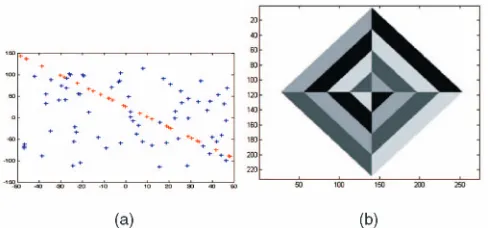
We chose the kernels k and k at pixel i as being Gaussian distributions. Consequently, the only parameters needed in our modeling are the expectation and the variance. Note that more complex kernels forandcan be estimated locally using steerable filters [29]. These would be more accurate in particular at corners. Fig. 3. Observations: a cloud of points,fðxi; yiÞgi¼1;100, and an image. (a) Sparse

cloud of points. (b) Imagediamond[15].

TABLE 1 Robustness

5

E

R

We compute a discrete representation of our estimatesp^ð; Þon

a fine grid2 ð₂::₂Þand2 ½l::þl.represents the

resolution of the discrete density on the axis and is the

resolution in the direction. These have been chosen as¼ =180

and¼1in the experiments Section 5.lis the maximum limit of

. Assuming an image of sizewhwith the origin of the spatial

coordinates in the middle of the image, then

l¼

ffiffiffiffiffiffiffiffiffiffiffiffiffiffiffiffiffiffiffiffiffiffiffiffiffiffiffi w

2 2

þ h

2 2 s

: ð24Þ

Once our estimates are computed, we want to assess how well they capture the alignment content of the observations. In the experiment described in Section 5.1, only one alignment occurs and we compare the accuracy of the detected maximumð;^^Þin each of our p.d.f. estimates ofpð; Þ.

The whole p.d.f. pð; Þ encodes the probability of aligned edges in an image, and not only its maxima. We propose in Section 5.2 to visualize the corresponding (dual) density estimate ^

pxyðx; yÞ in the spatial domain computed by inverse Radon transform of our estimates of pð; Þ. If our density estimates ^

pð; Þencode the alignment content of the image well, then their Inverse Radon Transform will reflect it in the spatial domain by enhancing straight edges and discarding the rest (e.g., nonedges and nonstraight edges).

5.1 Estimate^pð; jSxyÞ

N data pointsfðxi; yiÞgi¼1;N¼100are randomly generated:

. ni¼30 belongs to a straight line (10¼xcosð =8Þ þ ysinð =8Þwithx2 ½50; 50),

. while no¼70 outlier points are uniformly distributed (noþni¼N).

All of these data points have equiprobable priors pi¼N1 (P1), although the clouds of the observed points can also be interpreted as the result of an edge segmentation process in an image (P2).

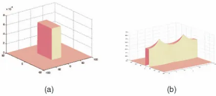
An example of the data is shown in Fig. 3a. The correspond-ing spatial densities p^xyðx; yjSxyÞ (see (15)) are computed with the variable bandwidth (VB) (Fig. 4a) (see (22)) and a fixed bandwidth (FB) in Fig. 4b with hxi¼hyi¼1; 8i. The corre-sponding densities p^ð; jSxyÞ are in Figs. 4c and 4d, and despite 70 percent of outliers, the maximum is easily detected to give a robust estimate of the line. Out of 100 simulations, 99 maxima ð;^^Þ of the density p^ð; jSxyÞ computed with a fixed bandwidth (FB1) were in the vicinity of the true values ð =8;10Þ with a precision of 1 degree for the angle and 1 for and 89 percent of the estimates with variable bandwidth (VB1). When relaxing the precision from 1 to 2 degrees and^¼102, all of the 100 estimates fð;^^ÞðnÞgcomputed with the fixed (FB2) and variable bandwidths (VB2) are found.

This experience is repeated for higher percentages of outliers (see Table 1). When the proportion of outliers reaches 90 percent, the fixed bandwidth gives a more reliable estimation of the line than with the variable bandwidth. Indeed, more prior information on the uncertainty of the observationsfðxi; yiÞgi¼1;N¼100is known when settinghxi ¼hyi¼1; 8i, and the estimated pdf is therefore better constrained.

5.2 Estimatesp^ð; jSÞandp^ð; jSxyÞ

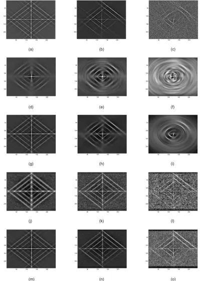
The imagediamondFig. 3b has been used in our experiment with three levels of noise N ð0; 2_{Þ with¼0; 20; 100. All of the} experiments use spatial Gaussian kernels with bandwidths hxi¼hyi¼1; 8i, for a prior P1 (all pixels have equiprobable priors). Fig. 5 shows the inverse Radon transform of our density estimates.FB(respectively,FB) indicates that the Sheather and Jones plug-in bandwidth [28] is used to set the bandwidths for and in computing ^pð; jSÞ (respectively,p^ð; jSxyÞ). The notationVB(respectively,VB) stands for variable bandwidths use for both and in computing p^ð; jSÞ (respectively, ^

pð; jSxyÞ).

Comparing Figs. 5a, 5b, and 5c, we can note that the weighted histogram renders a good alignment content for a moderate noise. Several straight contours with low contrast seem to disappear quickly as noise increases. The weighted histogram is an estimate of pðÞ that is fast to compute compared to the kernel-based

estimates. In fact, the weighted histogram can be seen as a truncated estimate ofp^ðjSÞ, where the tails of the Gaussian kernels are not taken into account.

Figs. 5d, 5e, and 5f compare the estimates p^ðjSÞ computed with a fixed bandwidth. Even with no additional noise, the rendering of the straight contours is not very good as all pixels contribute with the same bandwidth. In contrast, Figs. 5g, 5h, and 5i show a better alignment content recovered using variable bandwidths as proposed in this paper. However, as the noise increases, the reconstruction gets very bad: the variable bandwidth computed for the variable does depend on the noise level but also on the spatial position ðx; yÞ. As expected, as we go further away from the spatial origin (taken in the center of the image), the quality of the rendering of the straight contours deteriorates.

Figs. 5j, 5k, and 5l show the inverse Radon transform of the estimate ^pð; jSxyÞ computed with fixed bandwidth on the variable . The rendering reflects the alignment content of the image diamond well and does not deteriorate away from the spatial origin as for^pðjSÞ. This is even improved when using variable bandwidths in Figs. 5m, 5n, and 5o.

Fig. 6 presents the inverse radon transform computed on the estimates p^ð; jSxyÞ of two real images. Only the alignment content remains while strong contours from objects with no straight edges do not. While computing the inverse Radon transform of the estimates ofpð; Þhelps to visualize all the information encoded, many works on the Hough transform have only focused on detecting its modes (maxima) to recover the aligned segments (see Fig. 6). In [30], bumps are segmented inpð; Þas an alternative to modes, to recover the spatial alignments.

6

C

We have proposed several kernel modelings to generalize the Hough Transform. This new approach is unsupervised since all the needed bandwidths are automatically estimated. In addition, by explicitly modeling dependencies between the variables, we proposed a kernel modeling that is not depending on the choice of the origin of the coordinates in the spatial domain. The resulting density ^pðjSxyÞ encodes the alignment content of the images well and is robust to noise. Computing the Statistical Hough Transform on an image is more computationally expensive than the Standard Hough transform because all pixels of the image are used (instead of selecting only the edges) and, moreover, the tails of the kernels have to be taken into account in computing the estimates. Future work will investigate random and edge selection strategies to speed up the Statistical Hough Transform.

A

This work has been supported by the Enterprise Ireland Innova-tion Partnership IP-2006-412 and a Research Google Award.

R

[1] P. Hough, “Methods of Means for Recognizing Complex Patterns,” US Patent 3 069 654, 1962.

[2] R.O. Duda and P.E. Hart, “Use of the Hough Transformation to Detect Lines and Curves in Pictures,”Comm. ACM,vol. 15, pp. 11-15, Jan. 1972.

[3] J.-Y. Goulermas and P. Liatsis, “Incorporating Gradient Estimations in a Circle-Finding Probabilistic Hough Transform,” Pattern Analysis and Applications,vol. 2, pp. 239-250, 1999.

[4] A. Goldenshluger and A. Zeevi, “The Hough Transform Estimator,”The Annals of Statistics,vol. 32, no. 5, pp. 1908-1932, Oct. 2004.

[5] A.S. Aguado, E. Montiel, and M.S. Nixon, “Bias Error Analysis of the Generalized Hough Transform,”J. Math. Imaging and Vision,vol. 12, pp. 25-42, 2000.

[6] M. Bober and J. Kittler, “Estimation of Complex Multimodal Motion: An Approach Based on Robust Statistics and Hough Transform,”Image and Vision Computing J.,vol. 12, no. 10, pp. 661-668, Dec. 1994.

[7] P. Ballester, “Hough Transform and Astronomical Data Analysis,”Vistas in Astronomy,vol. 40, no. 4, pp. 479-485, 1996.

[8] G.R.J. Cooper and D.R. Cowan, “The Detection of Circular Features in Irregularly Spaced Data,”Computers & Geosciences,vol. 30, no. 1, pp. 101-105, Feb. 2004.

[9] C. Schmid, R. Mohr, and C. Bauckhage, “Evaluation of Interest Point Detectors,”Int’l J. Computer Vision,vol. 37, no. 2, pp. 151-172, 2000.

[10] B. Schiele and J.L. Crowley, “Recognition without Correspondence Using Multidimensional Receptive Field Histograms,” Int’l J. Computer Vision, vol. 36, no. 1, pp. 31-50, Jan. 2000.

[11] B.W. Silverman,Density Estimation for Statistics and Data Analysis.Chapman and Hall, 1986.

[12] D. Comaniciu and P. Meer, “Mean Shift: A Robust Approach Toward Feature Space Analysis,” IEEE Trans. Pattern Analysis and Machine Intelligence,vol. 24, no. 5, pp. 603-619, May 2002.

[13] R. Dahyot, P. Charbonnier, and F. Heitz, “Unsupervised Statistical Change Detection in Camera-in-Motion Video,” Proc. IEEE Int’l Conf. Image Processing,Oct. 2001.

[14] Q. Ji and R.M. Haralick, “Error Propagation for the Hough Transform,” Pattern Recognition Letters,vol. 22, pp. 813-823, 2001.

[15] A. Bonci, T. Leo, and S. Longhi, “A Bayesian Approach to the Hough Transform for Line Detection,”IEEE Trans. Systems, Man, and Cybernetics, vol. 35, no. 6, pp. 945-955, Nov. 2005.

[16] G. Lai and R.D. Figueiredo, “A Novel Algorithm for Edge Detection from Direction-Derived Statistics,”Proc. IEEE Int’l Symp. Circuits and Systems, vol. 5, pp. 37-40, May 2000.

[17] R. Dahyot, N. Rea, A. Kokaram, and N. Kingsbury, “Inlier Modeling for Multimedia Data Analysis,” Proc. IEEE Int’l Workshop Multimedia Signal Processing,pp. 482-485, Sept. 2004.

[18] R. Dahyot and S. Wilson, “Robust Scale Estimation for the Generalized Gaussian Probability Density Function,” Advances in Methodology and Statistics (Metodoloski zvezki),vol. 3, no. 1, pp. 21-37, 2006.

[19] P. Meer and B. Georgescu, “Edge Detection with Embedded Confidence,” IEEE Trans. Pattern Analysis and Machine Intelligence, vol. 23, no. 12, pp. 1351-1365, Dec. 2001.

[20] N. Aggarwal and W.C. Karl, “Line Detection in Image through Regularized Hough Transform,”IEEE Trans. Image Processing,vol. 15, no. 3, pp. 582-591, Mar. 2006.

[21] M.A. Fischler and R.C. Bolles, “Random Sample Consensus: A Paradigm for Model Fitting with Applications to Image Analysis and Automated Cartography,”Comm. ACM,vol. 24, no. 6, pp. 381-395, 1981.

[22] D. Walsh and A.E. Raftery, “Accurate and Efficient Curve Detection in Images: The Importance Sampling Hough Transform,”Pattern Recognition, vol. 35, pp. 1421-1431, 2002.

[23] A. Bandera, J.P.B.J.M. Pe´rez-Lorenzo, and F. Sandoval, “Mean Shift Based Clustering of Hough Domain for Fast Line Segment Detection,”Pattern Recognition Letters,vol. 27, pp. 578-586, 2006.

[24] R.S. Stephens, “Probabilistic Approach to the Hough Transform,”Image and Vision Computing J.,vol. 9, no. 1, pp. 66-71, Feb. 1991.

[25] P. Huber,Robust Statistics.John Wiley and Sons, 1981.

[26] R.M. Steele and C. Jaynes, “Feature Uncertainty Arising from Covariant Image Noise,”Proc. IEEE Conf. Computer Vision and Pattern Recognition, pp. 1063-1069, 2005.

[27] J. Princen, J. Illingworth, and J. Kittler, “A Formal Definition of the Hough Transform: Properties and Relationships,”J. Math. Imaging and Vision, vol. 1, no. 2, pp. 153-168, 1992.

[28] S.J. Sheather, “Density Estimation,”Statistical Science,vol. 19, no. 4, pp. 588-597, 2004.

[29] W.T. Freeman, “Steerable Filters and Local Analysis of Image Structure,” PhD dissertation, Massachusetts Inst. of Technology, 1992.

[30] R. Dahyot, “Bayesian Classification for the Statistical Hough Transform,” Proc. IEEE Int’l Conf. Pattern Recognition,Dec. 2008.