Parameters Optimization in Friction Surfacing
Godwin Barnabas
Department of Mechanical Engineering, Velammal College of Engineering and Technology, Madurai, India *Corresponding Author: [email protected]
Copyright © 2014Horizon Research Publishing All rights reserved
Abstract Surface engineering involves altering the
properties of the solid surfaces which could be different from those of the core material to reduce the degradation over time. These are also used to impart a wide range of functional properties, including physical, chemical, electrical, electronic, magnetic, mechanical, wear-resistant and corrosion-resistant properties at the required substrate surfaces. Almost all types of materials, including metals, ceramics, polymers, and composites can be coated on materials, similar or dissimilar.Keywords Polymers, Degradation, Wear-Resistant,
Ceramics, Surface Engineering1. Introduction
Surface engineering involves altering the properties of the solid surfaces which could be different from those of the core material to reduce the degradation over time. These are also used to impart a wide range of functional properties, including physical, chemical, electrical, electronic, magnetic, mechanical, wear-resistant and corrosion-resistant properties at the required substrate surfaces. Almost all types of materials, including metals, ceramics, polymers, and composites can be coated on materials, similar or dissimilar.
2. Principle of Friction Surfacing
In this process, rotating cylindrical consumable rod is fed against a substrate with axial force acting simultaneously on the rod. The frictional heat is generated between the substrate and the consumable rod. Once the rubbing end of the consumable rod is sufficiently plasticized, the substrate is traversed horizontally with respect to the vertical consumable rod. Material flow at the area of contact occurs due to the combined effect of axial load, rod rotational speed, and substrate traverse speed. As the substrate moves at a specific rate, the plasticized metal deposits over it. The vertical force consolidates the plasticized metal and results in the formation of a continuous and metallurgically bonded layer. The width and thickness of the track thus produced on
the substrate depend on mechatrode material and diameter as well as friction surfacing process parameters (axial force, mechatrode rotational speed and substrate traverse speed) and hence are called critical process parameters. Usually, the width is 0.9 times as the diameter of the mechatrode.
Figure1. Schematic of friction surfacing
The material properties such as thermal conductivity, sliding characteristics, plasticity and physical properties such as mechatrode diameters will influence the thickness of deposit. The presence of high contact stress between substrate and mechatrode, removes oxide films over the substrate surface. The process is, to a large extent, self cleaning and regulating.
3. Literature Review
H.Khalid Rafi, G.D.Janaki Ram, G.Phanikumar and K.Prasad Rao [1] studied the effects of traverse speed on the geometry, interfacial bond characteristics and mechanical properties of coatings .
M.Chandrasekaran, A.W.Batchelor and S.Jana [2] studied that mild steel bonded well with the substrate and there was evidence of interfacial compound formation whereas in case of stainless steel there was no evidence of mixing and coating.
stainless steel coating of mild steel leads to the formation of carbides in the stainless steel adjacent to the interface as a result of carbon migration from mild steel towards stainless steel.
J.John Samuel Dilip and G.D.Janaki Ram [4] studied the individual layers upto the thickness of 1mm to 2mm can be added up successively by friction deposition. A solid cylinder of 20mm diameter and 50mm height was successfully produced with austenitic stainless steel AISI 304.
H. Khalid rafi, N.Kishore babu, G.Phanikumar and K.Prasad Rao [5] studied the microstructural evolution of stainless steel AISI 304 on low carbon steel using optical microscopy, electron back scattered diffraction and transmission electron microscopy.
Ramesh Puli, E. Nandha Kumar and G.D. Janaki Ram [6] showed that the microstructure tests showed good hardness results when stainless steel is coated over mild steel. Bend and shear tests indicated excellent coating/substrate bonding.
J.Gandra, R.M.Miranda and P.Vilac [7] studied the influence of axial force, rotation and traverse speed on interfacial bond properties were investigated.
G.M. Bedford, V.I. Vitanov and I.I. Voutchkov [8] studied the mechanism of auto hardening of the mechatrode coating on substrate is studied.
B.Jaworski, G.M.Bedford, I.Voutchkov and V.I.Vitanov [9] studied the procedures for data collection, management and optimization of friction surfacing process and found that the thickness of the coated layer is typically between 0.5-3mm depending on the mechatrode material and diameter.
4. Formation of Orthogonal Array by
Taguchi Method
No. of parameters: 3No. of levels: 3
Selection of array: L9 (3 * 3) orthogonal array Table 1a.
Trial. No Load (kN) Axial Rotational Speed (rpm) Traverse Speed (mm/s)
T1 7 800 1.6
T2 7 1200 2.2
T3 7 1600 2.7
T4 8 800 2.2
T5 8 1200 2.7
T6 8 1600 1.6
T7 9 800 2.7
T8 9 1200 1.6
T9 9 1600 2.2
Here ‘L’ signifies the No. of levels and ‘9’ signifies the No.
of runs. Thus L9 array has 9 runs. A L9 array can be used to cover all combination of two parameters at three levels each. The general structure of the L9 array is as shown below:
The total no. of runs in the Taguchi method is nine with three replicates.
[image:2.595.311.552.193.407.2]The L9 array structure is substituted with the parametric values of the project at the respective cells to form the L9 array of the project for optimization.
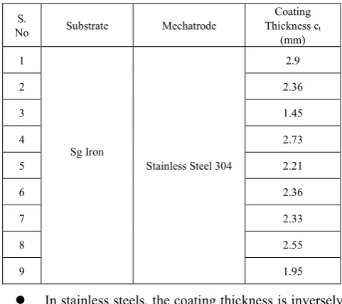
Table 1b. Coating Thickness (Ct) on Deposit Geometry
S.
No Substrate Mechatrode
Coating Thickness ct
(mm) 1
Sg Iron
Stainless Steel 304
2.9
2 2.36
3 1.45
4 2.73
5 2.21
6 2.36
7 2.33
8 2.55
9 1.95
In stainless steels, the coating thickness is inversely proportional to the traverse speed.
In higher traverse speed, the time of deposition of plasticized material on the work piece is less. Hence gives less coating thickness and less heat affected zone in work piece.
[image:2.595.311.553.193.397.2] Coating with minimum thickness is more advisable automobile parts applications. Higher coating thickness will give increase in weight of the component.
Table 1c.
S.
No Substrate Mechatrode Coating Width ct (mm)
1
Sg Iron Stainless Steel 304
19.72
2 16.83
3 14.49
4 18.9
5 17.29
6 16.14
7 19.23
8 19.44
Table 1d.
Trial. No A B C
T1 1 1 1
T2 1 2 2
T3 1 3 3
T4 2 1 2
T5 2 2 3
T6 2 3 1
T7 3 1 3
T8 3 2 1
T9 3 3 2
4.1. Coating Width (CW) on Deposit Geometry
The width of the flash formed in the substrate is usually 0.9 times the diameter of the mechatrode used.
Our results show approximately the same value.
4.2. OPTIMIZATION OF OUTPUT PARAMETERS Purpose of ANOVA
The purpose of the analysis of variance (ANOVA) is to investigate which design parameters significantly affect the quality characteristic. This is to accomplished by separating the total variability of the S/N ratios, which is measured by the sum of the squared deviations from the total mean S/N ratio, into contributions by each of the design parameters and the error. First, the total sum of squared deviations SST from the total mean S/N ratio nm can be calculated asSST =∑ (ni
–nm)2 where n is the number of experiments in the orthogonal
array and ni is the mean S/N ratio for the ith experiment.
4.3. Regression Analysis for Width The regression equation is
[image:3.595.58.306.77.303.2]D = 80.3 + 0.0123 A - 0.0374 B - 1.45 C
Table 1e.
Predictor Coef SE Coef T P
Constant 80.265 7.063 11.36 0.000
A 0.012275 0.003731 3.29 0.022
B -0.037379 0.003725 -10.04 0.000
C -1.4478 0.3725 -3.89 0.012
[image:3.595.63.506.78.360.2]S = 0.6873 R-Sq = 96.1% R-Sq(adj) = 93.8% Table 1f.
Term Coef SE Coef T P
Constant 23.89 0.0318 662.21 0.000
A 500 -0.3020 0.05182 -5.598 0.027
A 550 -0.0325 0.05182 -0.611 0.571
B 1750 0.8621 0.05182 15.119 0.006
B 1800 0.1701 0.05182 3.182 0.069
C 2.0 0.4188 0.05182 8.078 0.019
C 1.0 -0.1312 0.05182 -2.498 0.120
S = 0.1136 R-Sq = 97.3% R-Sq(adj) = 98.7% Analysis of Variance for SN ratios (Width)
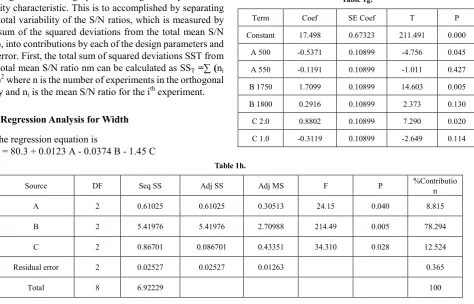
Table 1g.
Term Coef SE Coef T P
Constant 17.498 0.67323 211.491 0.000
A 500 -0.5371 0.10899 -4.756 0.045
A 550 -0.1191 0.10899 -1.011 0.427
B 1750 1.7099 0.10899 14.603 0.005
B 1800 0.2916 0.10899 2.373 0.130
C 2.0 0.8802 0.10899 7.290 0.020
C 1.0 -0.3119 0.10899 -2.649 0.114
Table 1h.
Source DF Seq SS Adj SS Adj MS F P %Contribution
A 2 0.61025 0.61025 0.30513 24.15 0.040 8.815
B 2 5.41976 5.41976 2.70988 214.49 0.005 78.294
C 2 0.86701 0.086701 0.43351 34.310 0.028 12.524
Residual error 2 0.02527 0.02527 0.01263 0.365
[image:3.595.74.549.457.761.2]S = 0.2504 R-Sq = 99.2% R-Sq(adj) = 98.3% Analysis of Variance for Means (Width)
5. Response Tables for S/N Ratio
(Width)
[image:4.595.314.551.121.321.2]Response table for Signal to Noise Ratios – Larger is better
Table 1i.
Level Axial Load Rotational Speed Traverse Speed
1 24.55 25.70 25.28
2 24.81 25.02 24.71
3 25.18 23.82 24.55
Delta 0.64 1.88 0.72
Rank 3 1 2
Based on the above table we can observe that the
rotational speed has contributed the most in affecting the width values and thus occupies the first position.
Response table for Means (Width)
[image:4.595.58.304.199.312.2]Graph 1. Table 1j.
Source DF Seq SS Adj SS Adj MS F P %Contribution
A 2 2.2840 2.2840 1.1420 18.26 0.032 8.396
B 2 21.2880 21.4880 10.6440 170.18 0.006 78.255
C 2 3.5060 3.5060 1.7530 28.03 0.034 12.888
Residual
error 2 0.1251 0.1251 0.0625 0.459
Total 8 27.2032 100
Table 1k.
Level Axial Load Rotational Speed Traverse Speed
1 17.01 19.28 18.43
2 17.44 17.85 17.25
3 18.27 15.55 17.00
Delta 1.22 3.73 1.43
Rank 3 1 2
Based on the above table we can observe that the rotational speed has contributed the most in affecting the width values and thus occupies the first position.
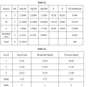
6. Main Effects Plot for Means
[image:4.595.156.472.340.646.2]Graph2.
The above graph (figure 7.1) shows the main effects plot for means where the optimum parameter will be based on the highest peak at each parameter. From the figure, it can be seen that highest width is obtained for 600 kg axial load, 1750 rpm rotational speed and 1.0 mm/s traverse speed.
7. Main Effects Plot for Signal to Noise
Ratio
Signal-to-noise ratio often abbreviated as SNR or S/N is a measure used in science and engineering to quantify how much a signal has been corrupted by noise. The SN ratio transforms several repetitions into one value which reflects the amount of variation present and the mean response.
[image:5.595.60.296.76.283.2]The above graph (figure 7.2) shows the main effects plot for the S/N ratio where the optimum parameter will be based on the highest peak at each parameter. From the figure it can be seen that width is obtained for 600 kg axial load, 1850 rpm rotational speed and 1.0 mm/s traverse speed.
Figure 2.
8. Contour Plot
In a contour plot, the values for two variables are represented on the x and y axes, while the values for a third variable are represented by shaded regions, called contours. A contour plot is like a topographical map in which x, y and z values are plotted instead of longitude, latitude and altitude.
The graph (figure2 ) shows the contour plot of width (in mm) vs. axial load (in N) and rotational speed (in rpm). It can be seen that maximum width can be obtained from minimum and maximum axial load and minimum rotational speed.
The graph (figure 3) shows the contour plot of width (in mm) vs. rotational speed (in rpm) and traverse speed (in mm/s). It can be seen that maximum width can be obtained until intermediate rotational speed and minimum and maximum traverse speed.
Figure 3.
[image:5.595.314.553.274.435.2]The graph (figure4) shows the contour plot of width (in mm) vs. axial load (in N) and traverse speed (in mm/s). It can be seen from the figure that maximum width can be found in minimum and maximum axial load and traverse speed.
[image:5.595.58.312.545.732.2]9. Residual Plot
Probability plot helps to determine whether a particular distribution fits your data or to compare different sample distributions. If the distribution fits the data:
The plotted points will roughly form a straight line. The plotted points will fall close to the fitted
distribution line.
Graph3.
[image:6.595.68.290.175.446.2]The (blue line) distribution line at the centre of the graph shows the desired width value in the normal probability plot. The trials (red dots) which lie close to the distribution line in the graph show the degree of closeness of the values.
Table 1l.
Trials Obtained Width Predicted Width
T1 19.72 19.45
T2 16.83 16.02
T3 14.49 14.12
T4 18.9 19.3862
T5 17.29 16.8443
T6 16.14 16.4543
T7 19.23 19.3296
T8 19.44 17.989
T9 16.04 16.1124
10. Predicted Width
From our experiment it is inferred that the obtained width and the predicted width are almost similar.
11. Optimization of Thickness
11.1. Regression Analysis for Thickness The regression equation is
D = - 3.77 + 0.00277 A + 0.00163 B - 0.0267 C Table 1m.
Predictor Coef SE Coef T P
Constant -3.7743 0.4973 -7.59 0.001
A 0.0027731 0.0002627 10.56 0.000
B 0.0016313 0.0002622 6.22 0.002
C -0.02668 0.02622 -1.02 0.356
S=0.752474 R-Sq = 96.8% R-Sq(adj) =94.9%
[image:6.595.311.553.211.331.2]11.2. Analysis of Variance for Thickness
Table 1n.
Source DF SS MS F P
Regression 3 85.960 28.653 50.06 0.000
Residual error 5 2.831 0.566
Total 8 88.7
Estimated Modal Coefficients for S/N ratio (Thickness) Table 1O.
Term Coef SE Coef T P
Constant 7.1487 0.2388 30.911 0.000
A 500 -0.5011 0.3219 -1.611 0.284
A 550 0.4988 0.3219 1.684 0.230
B 1750 1.3007 0.3219 4.077 0.059
B 1800 0.3667 0.3219 1.1209 0.401
C 2.0 1.1277 0.3219 2.990 0.067
C 1.0 0.1870 0.3219 0.603 0.619
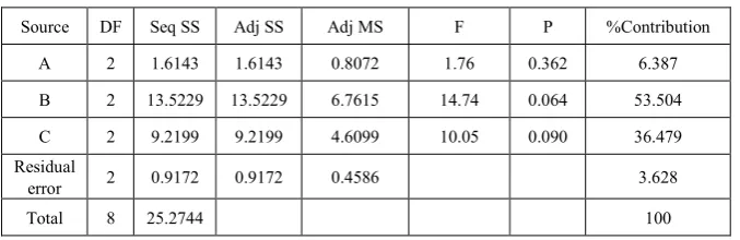
[image:6.595.313.553.384.495.2]Table 1p.
Source DF Seq SS Adj SS Adj MS F P %Contribution
A 2 1.6143 1.6143 0.8072 1.76 0.362 6.387
B 2 13.5229 13.5229 6.7615 14.74 0.064 53.504
C 2 9.2199 9.2199 4.6099 10.05 0.090 36.479
Residual
error 2 0.9172 0.9172 0.4586 3.628
Total 8 25.2744 100
[image:7.595.135.473.231.510.2]Estimated Modal Coefficients forMeans (Thickness)
Table 1q
Term Coef SE Coef T P
Constant 2.32599 0.02718 62.342 0.000
A 500 -0.08020 0.04215 -2.323 0.254
A 550 0.10813 0.04215 2.331 0.125
B 1750 0.33420 0.04215 4.324 0.032
B 1800 0.06754 0.04215 1.231 0.375
C 2.0 0.29488 0.04215 5.864 0.032
C 1.0 0.04201 0.04215 0.666 0.612
Table 1r
Source DF Seq SS Adj SS Adj MS F P %Contribution
A 2 0.06287 0.06287 0.03144 2.67 0.272 4.301
B 2 0.81891 0.81891 0.40945 34.79 0.028 56.022
C 2 0.55642 0.55642 0.27821 23.64 0.041 38.065
Residual
error 2 0.02354 0.02354 0.01177 1.610
Total 8 1.46174 100
11.3. Response Tables for S/N Ratio (Thickness) S = 0.1133 R-Sq = 92.4% R-Sq(adj) = 94.5% Analysis of Variance for Means (Thickness)
[image:7.595.138.476.594.703.2]Response table for Signal to Noise Ratios – Larger is better Table 1s
Level Axial Load Rotational Speed Traverse Speed
1 -5.620 -5.072 -3.811
2 -4.278 -3.929 -4.103
3 -1.974 -2.872 -3.959
Delta 3.646 2.201 0.292
Rank 1 2 3
Based on the above table we can observe that the rotational speed has contributed the most in affecting the thickness values and thus occupies the first position.
Table 1t
Level Axial Load Rotational Speed Traverse Speed
1 0.5262 0.5657 0.6621
2 0.6150 0.6480 0.6442
3 0.8006 0.7282 0.6355
Delta 0.2744 0.1625 0.0266
Rank 1 2 3
Based on the above table we can observe that rotational speed has contributed the most in affecting the thickness values and thus occupies the first position.
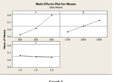
11.4. Main Effects Plot for Means
When performing a statistical analysis, one of the simplest graphical tools is a main effects plot. This plot shows the average outcome for each value of each variable, combining the effects of other variables.
Graph 4
The above graph4 shows the main effects plot for means where the optimum parameter will be based on the highest peak at each parameter. From the figure, it can be seen that highest thickness is obtained for 600 kg axial load, 1850 rpm rotational speed and 1.0 mm/s traverse speed.
Graph 5
12. Main Effects Plot for Signal to Noise
Ratio
Signal-to-noise ratio often abbreviated as SNR or S/N is a measure used in science and engineering to quantify how much a signal has been corrupted by noise. The SN ratio transforms several repetitions into one value which reflects the amount of variation present and the mean response.
[image:8.595.59.299.328.501.2]The above graph 5 shows the main effects plot for the S/N ratio where the optimum parameter will be based on the highest peak at each parameter. From the figure it can be seen that highest thickness is obtained for 600 kg axial load, 1850 rpm rotational speed and 1.0 mm/s traverse speed.
[image:8.595.60.298.582.737.2]Figure 5.
Figure 6.
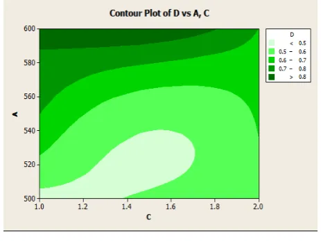
13. Contour Plot
In a contour plot, the values for two variables are represented on the x and y axes, while the values for a third variable are represented by shaded regions, called contours. A contour plot is like a topographical map in which x, y and z values are plotted instead of longitude, latitude and altitude.
from the figure that maximum thickness can be obtained at the maximum axial load and minimum rotational speed.
The Fig 6 shows the contour plot of thickness (in mm) vs rotational speed (in rpm) and traverse speed (in mm/s). It can be seen from the figure that the maximum thickness can be obtained at minimum rotational and traverse speed.
[image:9.595.62.294.205.379.2]The fig 7 shows the contour plot of thickness (in mm) vs. axial load (in N) and traverse speed (in mm/s). It can be seen that maximum thickness can be obtained at minimum traverse and axial load.
Figure 7.
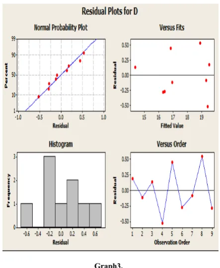
14. Residual Plot
Probability plot helps to determine whether a particular distribution fits your data or to compare different sample distributions. If the distribution fits the data:
The plotted points will roughly form a straight line. The plotted points will fall close to the fitted distribution line. Graph 6
The (blue line) distribution line at the centre of the graph shows the desired thickness value in the normal probability plot. The (red dots) which lie close to the distribution line in the graph show the degree of closeness of the values.
15. Predicted Thickness
Table 1u.
Trials Obtained Thickness Predicted Thickness
T1 2.9 2.03
T2 2.36 2.1198
T3 1.45 1.5986
T4 2.725 2.4568
T5 2.21 2.5520
T6 2.355 2.53036
T7 2.325 2.02856
T8 2.55 2.5836
T9 1.95 1.2265
From the above table it is inferred that the thickness obtained from our experiment is almost similar to the predicted thickness.
16. Conclusions
Experimental results show that the friction surfacing could be used as a method for obtaining coatings of dissimilar materials. Friction surfacing is the best method for obtaining deposits of stainless steel over ductile iron for critical applications. Adequate bond strength and good coating integrity of deposit is obtained by optimizing of process parameters. The deposit observed by the microscope showed dense, clear and fine microstructure of ferrite and pearlite on ductile iron side which clearly proves the superiority of the process. There were no cracks observed in the HAZ, showing the suitability of the parameters selected to give controlled heat input. Integrity of the deposit is excellent with good metallurgical bond.
REFERENCES
[1] G. Madhusudhan Reddy and T. Mohandas, “Friction Surfacing of Metallic Coatings on Steels”, Proceedings of the International Institute of Welding International Congress 2008, Chennai, India, January 2008, pp 1197 – 1213. [2] I. Voutchkov, B. Jaworski, V. I. Vitanov, and G. M. Bedford,
“An integrated approach to friction surfacing process optimization”, Surface and Coatings Technology, Vol. 141, 2001, pp 26-33.
[3] X. M. Liu, Z. D. Zou, Y. H. Zhang, S. Y. Qu and X. H. Wang, “Transferring mechanism of the coating rod in friction surfacing”, Surface and Coating Technology, Vol.202, 2008, pp 1889-1894.
[image:9.595.58.304.519.649.2][5] K. Prasad Rao, A. Veera Sreenu, H. Khalid Rafi, M.N. Libin and Krishnan Balasubramaniam, “ Tool steel and copper coatings by friction surfacing – A thermography study”, Journal of Materials Processing Technology, Volume 212, Issue 2, February 2012, Pp 402-407.
[6] Ramesh Puli and G.D. Janaki Ram, “Wear and corrosion performance of AISI 410 martensitic stainless steel coatings produced using friction surfacing and manual metal arc welding”, Surface and Coatings Technology, Volume 209, 25 September 2012, Pp 1-7.
[7] H. Khalid Rafi, G.D. Janaki Ram, G. Phanikumar and K. Prasad Rao, “Microstructural evolution during friction
surfacing of tool steel H1”, Materials & Design, Volume 32, Issue 1, January 2011, Pp 82-87.
[8] H. Khalid Rafi, G.D. Janaki Ram, G. Phanikumar and K. Prasad Rao, “Friction surfaced tool steel (H13) coatings on low carbon steel: A study on the effects of process parameters on coating characteristics and integrity”, Surface and Coatings Technology, Volume 205, Issue 1, 25 September 2010, Pp 232–242.