STUDIES ON IMPROVING TEXTURE SEGMENTATION PERFORMANCE USING GENERALIZED GAUSSIAN MIXTURE MODEL INTEGRATING DCT AND LBP

ISSN: 1992-8645 www.jatit.org E-ISSN: 1817-3195

SYNTHETIC RANGE IMAGE SIMULATION OF

TERRESTRIAL LIDAR SCANNER

1

THINAL RAJ, 2 FAZIDA HANIM HASHIM

1

Graduate Research Assistant, 2Senior Lecturer, Department of Electrical, Electronic and Systems

Engineering, Faculty of Engineering and Built Environment, The National University of Malaysia, Bangi

Malaysia

E-mail: [email protected], [email protected]

ABSTRACT

In recent years, the usage of Light Detection and Ranging (LiDAR) scanners has become predominant in the fields of robotics, navigation and remote sensing for numerous applications. Due to the high selling cost of LiDAR scanners, the research communities have developed LiDAR simulators mostly for Airborne Laser Scanning (ALS) application and some minimal works can be found for Terrestrial Laser Scanning (TLS) application. While the LiDAR simulators are becoming more sophisticated, there are still some applications area where the use of these simulators are not convenient. This paper describes an alternative and simple approach for developing a simulator for terrestrial LiDAR scanner application. The aim of this research is to model a synthetic 2D LiDAR scanner to provide range data based on object and sensor parameters input provided by the user. The object models are derived explicitly from geometrical relationships between the object and ray from scanner, thus avoiding the use of vectors. This approach directly raster the range image in contrast to ray tracing. The GUI-based simulator is developed in Processing language, thus it has an open source and hardware independent environment, making it ideal for research applications. The data obtained from this simulator can be used as ground truth for analyzing the characteristics of LiDAR scanners or can even be used for localization simulations.

Keywords: Terrestrial LiDAR, 2D Laser Scanner, Simulator, Range Image, Synthetic, Range Data

1. INTRODUCTION

Recently, range images obtained from Light Detection and Ranging (LiDAR) scanners have gained more popularity in the areas of remote sensing, navigation and robotics, at the expense of intensity images. Unlike intensity images acquired from cameras, the range data from laser scanners provides direct geometrical properties of scanned surface, which is stored as point cloud. The low post processing cost and complexity in obtaining geometry information are what make range data superior to intensity images.

Despite the high performance and capabilities of LiDAR scanners, the cost of the scanner can be significantly higher than that of a typical camera. For this reason, the research community has developed LiDAR simulators to provide synthetic range data based on object modeling. This effort significantly reduces the

research overhead for collecting range data. The LiDAR simulators are built on top of a notable computer graphics algorithm known as ray tracing, which is originally used for rendering photo realistic images. The main disadvantage of using ray tracing algorithm is that the computation is done pixel by pixel, thus slowing down the overall process. Modern GPU provides hardware acceleration to increase the performance of LiDAR Simulators to provide fast and accurate synthetic range data. While the simulators are getting more sophisticated, there are still some application areas where the simulator is not well suited. One such example is simulating 2D range data for Terrestrial Laser Scanner.

ISSN: 1992-8645 www.jatit.org E-ISSN: 1817-3195 JAVA-based environment known as Processing.

The basic assumption of the model is that the material at the surface of objects is perfect reflectors, thus the ray is not absorbed by it.

The results show that, our proposed models works efficiently in real-time in the Processing environment. The advantage of this simulator is that, the data can be readily utilized as ground truth for error analysis and calibration of LiDAR sensors.

The rest of the paper is organized as follows:

Section 2 discusses the framework and implementation on LiDAR scanner simulator in different platforms. Section 3 introduces the sensor model, object model as well as the implementation, while experimental results and discussions are presented in Section 4.

2. RELATED WORKS

Since the emergence of LiDAR sensors, researchers from various disciplines have conducted research on modeling and simulating synthetic range data. The simulated range data serves as ground truth for comparison against real scanned data. At a glance, LiDAR simulators can be classified based on the application area such as space exploration [1, 2], airborne simulation [3,4, 5], meteorology [6], and general terrain simulation [7].

The framework for simulating the range data are mostly based on a simple and well-known computer graphics technique known as ray tracing. However, the literature shows that the ray tracing algorithms were implemented using various platforms. For instance, [3] developed a LiDAR simulator in the JAVA platform for Airborne Laser Scanning application. In the preceding year, [8] and [9] implemented the LiDAR simulator in the CPP platform for Airborne Laser Scanning application and Terrestrial Laser Scanning application, respectively. Three years later, the same author of [8] improvised the simulator and implemented it in C# platform [10].

Implementing ray tracing-based LiDAR

simulator in higher level language slows down the rendering process, mainly because the CPU is not capable of executing the computations in parallel. An elegant solution to this problem can be seen at [11] whereby the LiDAR simulator was implemented in GLSL to directly access GPU resources such as vertex and fragment shader pipelines.

While the state of the art LiDAR simulators are fairly advanced, it is not specifically good enough for simulating 2D range data of Terrestrial Laser Scanner. The 2D range data is highly needed by the users of LiDAR scanners to calibrate and test the performance. In this paper, we propose an alternative approach to simulate 2D range data for various objects. The object models are derived explicitly based on geometrical relationships between the object and ray from scanner.

3. METHODOLOGY

3.1 Scanner Model

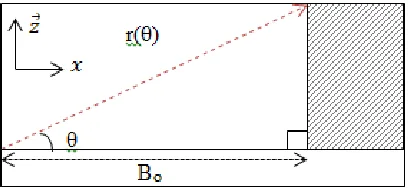
LiDAR scanners in the market exist in many varieties based on the intended application. The scanner described in this paper is based on a Pulselight3D V2 1D LiDAR. The specification of this scanner is shown in Table 1. The model assumes that scanning begins at 0 degrees before proceeding to move in an anti-clockwise direction until it reaches 180 degrees. Based on Figure 1, the condition for the scanner to detect the object is that the angle between the transmitted ray and the normal to the surface must be acute. If the ray is perpendicular to the normal to the surface, it would not detect the object.

Table 1: Specifications of Pulselight 3D v2

Specifications Unit

Max range 40 m

Accuracy +/- 2.5 cm

Beam Divergence 4 mRad

ISSN: 1992-8645 www.jatit.org E-ISSN: 1817-3195

Figure 1: scanner and object in local coordinate frame.

3.2 Model Assumptions

Models are only representations of real world phenomena under well-defined assumptions. The more assumptions made, the less accurate will the model be. The followings describe the assumptions made for the simulator:

1. The object is a perfect reflector, thus it does not diffract or absorb the incident ray from the scanner.

2. The scanner is always positioned at the center of the object, thus making the range data symmetrical about the center of coordinate.

3. The effect due to beam divergence is negligible.

4. The scanner only accepts single intensity return, meaning that it only measures the nearest distance between the scanner and the object. Multiple return distances due to reflection, diffraction or interference is assumed to be negligible.

3.3 Infinite Horizontal Object Model

The infinite horizontal object can be conceived as scanning a straight long wall. Figure 2 shows the illustration of a vertical object scanned in sensor coordinate frame. If the perpendicular distance H between the scanner and the object is known, then Equation 1 can be applied to compute the measured distance as a function of scan angle.

Figure 2: Distance observed by LiDAR scanner from top view

r (θ) = H × sec(θ) { θ : 0 < θ < π } (1)

3.4 Infinite Vertical Object Model

The long vertical sides of skyscrapers best describe infinite vertical objects. Similar to the previous case, if the horizontal distance Bo between the sensor and the object are known, then it is sufficient to find the relationship between the measured distance and the scan angle as shown in Equation 2. Figure 3 shows the object model in scanner coordinate frame.

Figure 3: Distance observed by LiDAR scanner from right view

r (θ) = B0 × cosec(θ), { θ : 0 ≤ θ < 0.5π} (2)

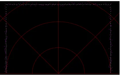
3.5 Rectangular Object Model

The rectangular object can be modeled as a piece-wise function by combining equation 1 and equation 2. Equation 3 shows the resulting piece-wise function for scan angle 0 to 180 degrees. The domain for the function can be computed using Equations 4 & 5. Since the object is symmetrical about the scanner coordinate frame as shown in Figure 4, the remaining problems can be further simplified by exploiting these properties. Therefore the final piece-wise functions are shown in

ISSN: 1992-8645 www.jatit.org E-ISSN: 1817-3195

Figure 4: Distance observed by LiDAR scanner from right view

θ1 = tan -1(2H/B0 ) (4)

θ2 = π - θ1 (5)

r1 (θ) = 0.5×B0 × cosec(θ), { θ : 0 ≤ θ ≤ θ1} (6)

r2(θ) = H × sec(θ), { θ : θ1 ≤ θ ≤ θ2} (7)

r3(θ) = - f1(θ) { θ : θ2 ≤ θ ≤ π} (8)

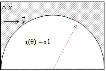
3.6 Circular Obstacle Model

Circular objects have a unique property compared to other geometries that is the radius of a circular object is always constant from its center as illustrated in figure 5. If the laser scanner is placed at its center, the distance measured is the radius of the object. Equation 5 describes the relationship between distances measured and scan angle.

Figure 5: circular plane observed by LRF from top view

r (θ) = r1, { θ : 0 ≤ θ ≤ π } (9)

3.7 Inverted Circular Obstacle Model

Straight pipes and tubes are real world examples of inverted circular objects. From the top view, these objects appear to be a circle, as illustrated in Figure 6.

A few properties of geometry have to be considered before deriving the geometrical relationships of these objects. Firstly, as stated before, while the transmitted ray is not perpendicular with the normal to the surface of an object, it is visible to the LiDAR scanner. Equation 10 represents the ray from the scanner while Equation 11 represents the object. By solving Equations 10 and 11 simultaneously, Equation 12 can be obtained. The discriminant of this quadratic equation describes the intersection between the line and the curve. The condition for the line and the circle to tangent can be computed using Equation 13. Solving Equation 13 yields Equation 14. Finally, the relationship between the measured distance and the scan angle are shown in Equations 15, 16 & 17 as piecewise functions.

Figure 6: circular object observed by LRF from top view

Figure 7: detail view of scanner ray (red) touches the circular object at tangent at point m

y= tan(θ)x (10)

x2 + (y-ao)2 = ab2 (11)

ISSN: 1992-8645 www.jatit.org E-ISSN: 1817-3195 (– 2a×tan(θ))2 - 4×sec2(θ)×( ab2- ao2) = 0 (13)

θ = β = cos-1(ab/ao) (14)

r1 (θ) = d × cosec(θ), { θ : 0 ≤ θ ≤ β} (15)

r2(θ) = ao × cosec(θ) + ab , { θ : β< θ < π-β} (16)

r3(θ) = - f1(θ) { θ : π-β≤ θ ≤ π} (17)

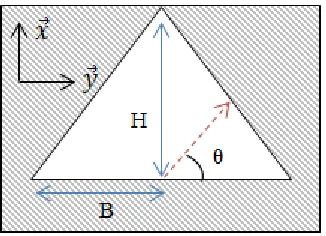
3.8 Triangular Obstacle Model

Edges of walls are good representations of triangular objects. Figure 8 shows the illustration of a triangular object in scanner coordinate frame. Equation 18 is the linear equation representing the wall. By solving Equations 18 and 10 simultaneously, the relationship between the measured distance and the scan angle can be obtained as shown in Equation 19. Notice that Equation 19 returns an error when the scan angle is equal to 90 degrees. Therefore Equations 20, 21 & 22 are the final piecewise functions which include the exception at 90 degrees.

Figure 8: Triangular object observed by laser scanner from top view.

y = (-H/B)x + H (18)

r(θ)= H×B×sec(θ)/ (H + B×tan(θ)) (19)

r1 (θ) = H×B×sec(θ)/ (H + B×tan(θ)),

{ θ : 0 ≤ θ < 0.5π } (20)

r2(θ) = H { θ : θ = 0.5π } (21)

r3(θ) = - f1(θ) { θ : 0.5π < θ ≤ π } (22)

3.9 Inverted Triangular Object

Inverted triangular objects are rarely found in the real world. However they are easy to construct and can be utilized for testing the performance of a LiDAR scanner. Figure 9 shows the illustration of an inverted triangular object in sensor coordinate frame. The derivation of measured distance as a function of scan angle is shown in Equations 23, 24 & 25 which undergoes a similar process as the triangular object.

Figure 9: Inverted Triangular object observed by laser scanner from top view.

r1 (θ) = H×B×sec(θ)/ (H - B×tan(θ)),

{ θ : 0 ≤ θ < 0.5π } (23)

r2(θ) = H { θ : θ = 0.5π } (24)

r3(θ) = - f1(θ) { θ : 0.5π < θ ≤ π } (25)

3.10 Coordinate Transformation

All the functions described earlier exist in polar coordinate form. Conversion from polar to Cartesian coordinate can be done using Equations 26 and 27.

x = r (θ) ×cos(θ) (26)

y = r (θ)×sin(θ) (27)

3.11 Implementation

ISSN: 1992-8645 www.jatit.org E-ISSN: 1817-3195 the simulator more attractive, a GUI is developed

using the Processing library.

lidarSim Height: float

Base: float

Radius: float

ObserverHeight: float

minAngle: float

maxAngle: float

stepSize: float

gridx: int

gridy: int

infHorizon(min,max,step,H,) infVertical(min,max,step,B) Rect(min,max,step,B,H) Circ(min,max,step,R) invCirc(min,max,step,R,OH) trig(min,max,step,B,H,OH) invTrig(min,max,step,B,H,OH) grid(gx,gy)

Figure 10: class diagram of lidarSim class.

Figure 11: Flow Chart Of The Lidar Simulator Program.

4. RESULTS & DISCUSSIONS

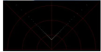
All the methods from lidarSim class are tested one by one for the scan angle beginning from 0 to 180 degrees. Figures 12 and 13 show the results obtained for an infinite horizontal object with Height = 100 and an infinite vertical object with Base = 100cm, respectively. In Figure 13, it is noticed that the scan points are denser for more acute angles. Figure 14 shows the results obtained for a rectangular object with Height = 200cm & Width = 100cm while Figure 15 shows the results obtained for a circular object with 100cm radius.

The results for an inverted circular object with radius 100 cm is illustrated in Figure 16. The scan results in Figure 16 reveals that, as the distance between the scanner and the object decreases, only a small portion of the object can be observed by the scanner. Figures 17 and 18 show the result obtained for triangular objects. In real circumstances, the corners of the wall are not perfectly sharp, thus it’s impossible to obtain a perfect scan. However, it is possible to setup a rectangular surface in lab scale to test the performance of scanners at sharp corners. Furthermore, the scanners are unable to detect rays coming from sharp objects like the inverted triangle. This is because the transmitted ray from the LiDAR scanner will be greatly diffracted by sharp objects in reality.

Figure 19 illustrates the effect of the scan angle step size on an infinite vertical object. The simulation was tested for step sizes of 0.5o, 1.0o, 1.5o, 2.0o & 5.0o. Clearly it can be observe that the step size affects the quality of the scan. If the LiDAR scanner scans an uneven rough surface with a large step size, it will most likely miss the geometric identity of the surface. In practice, there is always a trade off between the step size, the quality of the scanned data and the time required for the scan. Small step angles provide a high quality data, but in return it requires more time to complete the scan.

ISSN: 1992-8645 www.jatit.org E-ISSN: 1817-3195 representing the corrupted data of +/- 2.5 cm and

the blue points as the ground truth. The built-in random number generator function in Processing generates the measurement error according to the manufacturer’s specifications. Although the pseudo random is an approximate solution, the efficiency of this generator can be improved by assigning a large seed value to it.

Figure 12: Horizontal object scan simulation

for H=100cm

Figure 13: Vertical object scan simulation for B=200cm

Figure 14: Rectangular object scan simulation for B=200cm & H=100cm

Figure 15: Circular object simulation for radius = 100 cm

Figure 16: Inverted circular object simulation for radius = 100 cm observed at h=50 cm away from the object

Figure 17: Triangular object simulation for B=100cm and H = 200cm

ISSN: 1992-8645 www.jatit.org E-ISSN: 1817-3195

Figure 19: The effect of infinite vertical objects scanned at step angle 0.5o(green), 1.0o(yellow), 1.5o(blue),

2.0o(magenta), 5.0o(white)

Figure 20: The effect of measured error (magenta) and ground truth (white) for rectangular object.

One advantage of implementing the simulators in Processing environment is that it simulates fast and real time. This is because the P2D graphics renderer used in Processing makes use of OpenGL library compatible graphics hardware. However the readers are encouraged to implement the model in different environments. In addition to that, the source code of the simulator can be exported as a stand-alone application. This improves the usability of the simulator.

5. CONCLUSIONS & FUTURE WORKS

The simulator proposed in this paper imitates the behavior of 1D and 2D LiDAR scanners available in the market to generate synthetic range data. The user can change the desired object model and tweak the parameters to generate range data without any complications. Besides that, an additional accuracy parameter is provided to simulate the measurement uncertainty of LiDAR scanners. The simulator with a user friendly GUI was fully developed in an open source and

hardware independent environment known as Processing so that it can be easily utilized by the public.

The synthetic range data obtained from the simulator are mainly used by surveyors or researches as ground truth to analyse the performance of LiDAR scanners. Moreover, the simulators can be used for education purposes to study the characteristics of LiDAR without having to purchase an actual scanner.

One drawback of our sensor model is that, it assumes the material of the object is isotropic. Therefore the scan is only dependent on the geometry of the object regardless of the properties of the material. In the future, we would like to include the effects of properties of materials to improve the accuracy of the simulator.

REFRENCES:

[1] Parkes, S., I. Martin, M. Dunstan, Planet Surface Simulation with PANGU. In Eighth International Conference on Space Operations, 2004

[2] Fochesattoa, J., P. Ristoria, P. Flamantb, M. E. Machadoc, U. Singhd, E. Quel, Backscatter LIDAR signal simulation applied to spacecraft LIDAR instrument design. Advances in Space Research, 2004, vol. 34(10), pp. 2227-2231. [3] Lohani, B., R. K. Mishra, Generating LiDAR

data in laboratory: LiDAR simulator. International Archive of Photogrammetry and Remote Sensing, 2007, vol. XXXVI(3).

[4] Gillespie, J. B., E. M. Patterson, UVTRAN: An Ultraviolet Transmission and Lidar Simulation Model. Tech. Rep. ADA317395, Army Research Lab White Sands Missile Range NM, 1996. [5] Streicher, J., I. Leike, LabVIEW software for

lidar simulation. In J.-P. Wolf, ed., Proc. SPIE, Lidar Atmospheric Monitoring, 1997, vol. 3104, pp. 285-289.

[6] de Boer, G., Nested High Resolution Simulation and LiDAR Validation of a Land Breeze Circulation. Master's thesis, University of Wisconsin - Madison, Department of Atmospheric and Oceanic Sciences, 2004. [7] Brown, S. D., D. D. Blevins, J. R. Schott,

ISSN: 1992-8645 www.jatit.org E-ISSN: 1817-3195 [8]Kim, S., Min, S., Kim, G., Lee, I., & Jun, C.,

Data Simulation of an Airborne LIDAR System. Proceedings of SPIE - The International Society for Optical Engineering, 2009, 7323(1), pp. 1– 10.

[9] Doria, D., A Synthetic LiDAR Scanner for VTK. The Insight Journal, 2009, pp. 1–9.

[10] Kim, S., Lee, I., & Lee, M. Lidar Waveform Simulation Over Complex Targets. ISPRS - International Archives of the Photogrammetry, Remote Sensing and Spatial Information Sciences, 2012, XXXIX-B7 (September), pp. 517–522.