ORIGINAL RESEARCH ARTICLE
ON NUMERICAL SOLUTIONS OF FUZZY DIFFERENTIAL EQUATIONS
*1
Kodal Sevindir, H.
1Cetinkaya, S. and
2Tabak, G.
1
Kocaeli University, Department of Mathematics, Kocaeli, TURKEY
2
Kocaeli University, Mathematics Graduate Program, Kocaeli, TURKEY
ARTICLE INFO ABSTRACT
Controlling After being introduced by Chang and Zadeh, the topic of Fuzzy Differential Equations has been attracting a rapidly growing number of researchers in recent decades. In this paper some numerical algorithms for fuzzy ordinary differential equations are considered. Schemes for the classical Euler method, Homotopy Analysis Method (HAM), and Adomian Decomposition Method (ADM) are discussed; this is followed by an error analysis. The algorithms are used to solve numerically for a linear fuzzy Cauchy problem, and the first two iterative steps of the algorithms are shown explicitly in detail.
Copyright © 2018,Kodal Sevindir et al. This is an open access article distributed under the Creative Commons Attribution License, which permits unrestricted use, distribution, and reproduction in any medium, provided the original work is properly cited.
INTRODUCTION
Fuzzy differential equations naturally represent dynamical systems with uncertainty. Therefore, this theory has an important role in science and engineering. Dubois and Prade introduced the concept of fuzzy derivative using the extension principle in (Abu Arqub, 2013). Kaleva (Kaleva, 1987) and Seikkala (Seikkala, 1987), then formulated Fuzzy differential equations in time dependent form. In (Liao, 1992), Liao used the basic ideas of homotopy in topological concept to offer an analytic method for nonlinear problems [15-18]. Fuzzy Initial Value Problems (FIVPs) may not always have solutions which can be obtained via analytical methods. Because of this difficulty, numerical methods are used to approximate the solutions of such problems. (Abu Arqub, 2013). Numerical methods have been succesfully applied to some fuzzy differential equations provided that the necessary conditions are satisfied. The numerical solvability of fuzzy differential equations can be found in (Abu Arqub, 2013; Abu Arqub, 1903; Abbasbandy, 2002; Abbasbandy, 2006; Allahviranloo, 2009; Babolian, 2004; Effati, 2010; Ma, 1999; Ch. Palligkinis, 2009; Shokri, 2007; Rabie, 2013) and references therein. In this paper we present explicitly numerical approximation steps to the solution of a FIVP via Euler method, homotopy analysis method (HAM), and Adomian decomposition method (ADM) algorithms, and compare the numerical results obtained.
Preliminaries
In this section, we introduce some necessary definitions and preliminary results from fuzzy calculus theory. We will utilize Hukuhara differentiability for the concept of fuzzy derivative.
Let ≠ ∅ be a set. A fuzzy set in is characterized by its membership function : → [0,1].
*Corresponding author: Kodal Sevindir, H.
Kocaeli University, Department of Mathematics, Kocaeli, TURKEY
ISSN: 2230-9926
International Journal of Development Research
Vol. 08, Issue, 09, pp.22971-22979, September,2018
Article History: Received 14th June, 2018
Received in revised form 20th July, 2018
Accepted 19th August, 2018
Published online 30th September,2018
Key Words:
Fuzzy differential equations, Fuzzy Cauchy problem,
Euler method, Homotopy Analysis Method, Adomian Decomposition Method.
Citation: Kodal Sevindir, H. Cetinkaya, S. and Tabak, G. 2018. “On numerical solutions of fuzzy differential equations”, International Journal of Development Research, 8, (09), 22971-22979.
Definition (Goetschel, 1986 and Kaleva, 1987),A fuzzy number is a fuzzy subset of the real line with a convex, normal, and upper semicontinuous membership function of bounded support.
The set of all fuzzy numbers is denoted by .
Definition (Ebadian, 2017) For any ∈ the r -cut set of is denoted by [ ] and defined by [ ] = x ∶ μ ( x ) ≥ r, xϵX , where 0 ≤ ≤ 1. The notation [ ] = [ , ] , 0 ≤ ≤ 1 refers to the lower and upper branches on . Alternatively definition of fuzzy numbers can be given in the parametric form as follows:
Definition (Kaleva, 1987) An arbitrary fuzzy number in parametric form is an ordered pair of functions ( ( ), ( )), 0 ≤ ≤ 1, which satisfy the following three conditions:
(i) ( ) is a bounded monoton increasing left continuous function on (0,1] and right continuous at 0. (ii) ( ) is a bounded monoton decreasing left continuous function on (0,1] and right continuous at 0. (iii) ( ) ≤ ( ), 0 < < 1.
There are a few derivative varieties in the study of fuzzy differential equations:
Hukuhara differentiability
Seikkala differentiability
Strongly generalized differentiability
In this paper we consider Hukuhara differentiability. The differentiability in the sense of Hukuhara (H-derivative) for fuzzy functions are based on the H-difference of sets.
Definition [9] Let : [ , ] → ℱ (ℝ ). Let x, y ∈ ℝ be two fuzzy numbers. If there exists a fuzzy number z ∈ ℝ such that
x = y + z then is called Hukuhara difference (H-difference) of and , and it is denoted by z = xΘ y.
Definition [23] Let : [ , ] → ℱ (ℝ ). If for sufficiently small h>0 there exist H-differences ( + ℎ) ( ) and
( ) ( + ℎ) such that
→
( ) ( )
= →
( ) ( )
= ′( )
, ……….(1)
then the Fuzzy number ′( ) is said to be Hukuhara derivative of the function at a point .
2. Fuzzy Initial Value Problem
If any parameter in an initial value problem (2) has fuzziness, then the problem becomes a fuzzy initial value problem (3) [14,24].
´( ) = ( , ( ))
(0) = ………...(2)
´( ) = , ( ) ,
( ) = ∈ [ , ] ………...………(3)
where r-cuts are [ ] = [ (0; ), (0; )], (0,1].
Following Zadeh’s extension principle, for = ( ) we can write
( ) ( ) = sup{ ( ): = ( )} , ∈ ℝ}. Thus we will have
[ ( ( ))] = [ ( ; ), ( ; )], (0,1]
where
( ; ) = min ( ): ∈ ( ; ), ( ; ) ,
( ; ) = max ( ): ∈ ( ; ), ( ; ) .
Derivative of a fuzzy function ( ) can be defined as [24]:
[f´ y(t) ] = [ ′(y; r), ′(y; r)], ∈ , ∈ (0,1]
where
′(y; r) = min
′( ): ∈ ( ; ), ( ; )
′(y; r) = max
′( ): ∈ ( ; ), ( ; )
To have a unique solution for FIVP (2), must satisfy Lipschitz condition:
∥ ( ) − ( ) ∥ ≤ ∥ − ∥, ≥ 0.
For (0,1] the equivalent system to problem (3) can be written as
´(t, r) = ( ) = ( ; ) = ( ; ), ( ; ) , ……….(4)
(0, ) = ( ), ………..(5)
´(t, r) = ( ) = ( ; ) = ( ; ), ( ; ) , ……….…….(6)
(0, ) = ( ). [14] ……..………..(7)
Definition Let : ( , ) → and x ∈ ( , ). (i) If for sufficiently small ℎ > 0, ∃ ( + ℎ) ( ), ∃ ( ) ( − ℎ) such that → ( ) ( ) = → ( ) ( ) = ′( ) holds, then is said to be (1) – differentiable. (ii)If for sufficiently small ℎ > 0, ∃ ( + ℎ) ( ), ∃ ( ) ( − ℎ) such that → ( ) ( ) = → ( ) ( )= ′( )holds, then is said to be (2) – differentiable. Theorem Fora function : → (ℝ) and for ∀ ∈ [0,1] we can define r-cuts as [ ( ; )] = [ ( ; ), ( ; )]. That is, (i) If is (i) – differentiable then ( ; ) and ( ; ) are differentiable functions and [ ′( ; )} = [ ′( ; ), ′( ; )] (ii) If is (ii) – differentiable then ( ; ) and ( ; ) are differentiable functions and [ ′( ; )} = ′( ; ), ′( ; ) . 3. Numerical Solutions of a Fuzzy Initial Value Problem Consider the first order Fuzzy Initial Value Problem (3). In (3), is a fuzzy function of ; ( , ( )) is a fuzzy function of a variable and a fuzzy variable ; ′ is the Hukuhara derivative of . Initial condition ( ) = may be a fuzzy number. In this paper we solve a FDE via three numerical methods: Euler method, Adomian method and Homotopy Analysis Method. Euler Method Euler method uses the first order term of the Taylor series to find an approximate solution of a differential equation. Consider the FIVP (3). Parametric form of (3) can be written as (4-6). To integrate (4) and (6), we partition the interval [ , ] into M equal pieces: ( < < < ⋯ < = ). Let us denote the exact solution of FIVP as [Y(t)] = [Y(t; r), Y(t; r)]and the approximate solution as [y(t)] = [y(t; r), y(t; r)]. In this case, the exact solution is (r) = [ (r), Y (r)] and the approximate solution is (r) = [ (r), y (r)] at where 0 ≤ ≤ 1. Here = + ℎ, ℎ = 1 ≤ ≤ . Similar to the classical case, the Euler Method for the fuzzy problem uses the first order approximates of Y′(t; r) and Y(t; r), and can be written as ′( ; ) ≈ ( ; ) ( ; ). ………..……….(8)
Here Z(t;r) can alternatively be taken as Y(t; r) and Y(t; r).
Using (8) we obtain
(r) = (r) + ℎ (r)
Y (r) = Y (r) + h (r)
Where
(r) ≜ , (r), Y (r) and from here we get (r) = (r) + ℎ , (r), y (r)
y (r) = y (r) + ℎ , (r), y (r) .
3.2. HAM yöntemi
Let us consider the following differential equation [ ( )] = 0, ≥ , where denotes a nonlinear differential operator and
( ) denotes an unknown function of . The 0th-order deformation equation can be written as [15]
(1 − )ℒ[ ( ; ) − ( )] = ℏ ( ) [ ( ; )]. ……….……….(9)
Here ∈ [0,1] is the embedding parameter, and ℒ is an auxiliary linear operator such that
ℒ[ ( )] = 0 when ( ) = 0.
In (9), ( ; ) denotes the unknown function, ( ) is an initial value for , ℏ ≠ 0 is an auxiliary parameter, and ( ) ≠ 0
represents an auxiliary function. As q increases from 0 to 1, the solution (t;q) varies continuously from the initial approximation to the exact solution.
The mth-order deformation derivative is defined as
( ) = !
( ( ; )
. We then expand the solution function ( ; ) in a Taylor series with respect to the embedding
parameter q;
( ; ) = ( ) + ∑∞ ( ) .
In this paper, we consider the construction of solution for fuzzy IVPs with respect to (1)- differentiability via HAM. The (2)-differentiability case is similar to this one. For the fuzzy case the Homotopy method is based on continuos mappings ( ) → ( ; ) and ( ) → ( ; ). Similar to the regular ODEs, as the embedding parameter q varies from 0 to 1, the functions
( ; ) and ( ; ) varies from an initial approximation to the exact solution.
We then define
[ ( ; )] = [ ( ; ) − , ( ) , ( ; ), ( ; ) ,
[ ( ; )] = [ ( ; ) − , ( ) , ( ; ), ( ; )
where and are nonlinear operators. Using q, we can assemble a family of 0th-order deformation equations
(1 − )ℒ ( ; ) − , ( ) = ℏ ( ) ( ; ) ,
(1 − )ℒ ( ; ) − , ( ) = ℏ ( ) ( ; ),
subject to the initial conditions ( ; ) = , ( ) and ( ; ) = , ( ). Here , ( ) and , ( ) are the initial
approximations of ( ) and ( ), respectively.
We obtain Taylor expansion for ( ; )and ( ; ) of q as
( ; ) = , ( ) + ∑∞ , ( )
( ; ) = , ( ) + ∑∞ , ( )
where , ( ) and , ( ) are given, respectively, as !
( ; )
and
!
( ; )
. Thus, when q = 1, the series becomes
( ) = , ( ) + ∑∞ , ( ), ( ) = , ( ) + ∑∞ , ( )
From the mth-order deformation equations, we have
ℒ , ( ) − , ( ) = ℏ ( )ℜ ⃗ ( ), ⃗ ( ) ,
Where
ℜ ⃗ ( ), ⃗ ( ) = , ( ) −( )!
, [ , ( ; ), ( ; )]
→
ℜ ⃗ ( ), ⃗ ( ) = , ( ) −( )!
, [ , ( ; ), ( ; )]
→
.
When we choose ( ) = 1,ℏ = ℏ, and ℒ = , for = 1,2, the right inverse of will be the integral ∫ (. ) . Hence, the mth -order deformation equation for ≥ 1 can be written as
, ( ) = , ( ) + ℏ ∫ ℜ ⃗ ( ), ⃗ ( ) ,
, ( ) = , ( ) + ℏ ∫ ℜ , ⃗ ( ), ⃗ ( ) .
If we choose , ( ) = ( ) = and , ( ) = ( ) = as initial guesses of ( ) and ( ), respectively, we can
calculate ,( ) and ,( ), i= 1,2, … , by using the iteration formula above. Ultimately, we find the approximate solution ( ) and ( ) of the corresponding system via the series
, ( ) = ∑ , ( ), , ( ) = ∑ , ( ).
A special case of HAM is the Adomian Decomposition Method which will be briefly explained in the next subsection.
3.3. Adomian Decomposition Method
The Adomian decomposition method, introduced by Adomian in the 1980s, can be used to solve linear and nonlinear equations [5, 6]. To solve a nonlinear functional equation of the form − ( ) = where is the given function and is the nonlinear operator, we consider the solutions = ∑∞
in the series form. Here the nonlinear operator is of the form ( ) = ∑∞ ,
and polynomial in , , … , are called Adomian polynomials.
Let
= ∑∞
,
(∑∞ ) = ∑∞
and
= ( ),
= ( ),
= ( ) + ( /2!)( / ) ( ),
= ( ) + ( ) ( ) +
! ( ),
…
=
! [ (∑
∞ )] , = 0,1,2, …
where is a parameter. The iterative formula
= ( , , … , ),
= 0,1,2, …
= ……….(50)
is used to determine the terms of the series
= ∑∞ .
Truncated series Ψ = + + ⋯ + is then used to approximate .[6, 8]
4
. RESULTS AND DISCUSSION
Example: Consider the fuzzy initial value problem
′( ) = − ( ) + sin ( ),
(0) = 24
25+
1 25 ,
101
100−
1
The exact solution is
( ) = ( ( ) − ( )) + + + , ( ( ) − ( )) + + + .
Now let us show the first a few approximate solution steps explicitly for all three methods.
a) Via Euler method: Using Euler method we write the iterative equations
(r) = (r) + ℎF , (r), y (r) ,
y (r) = y (r) + ℎG , (r), y (r) ,
with
(0; ) = + , (0; ) = − ,
where = 1,2,3, … , − 1 and ℎ = ,
then we obtain
= + ℎ − + sin( ) =24
25+
1
25 + ℎ −
24
25−
1
25 + sin( )
= + ℎ − + sin( ) =24
25+
1
25 + ℎ −
24
25−
1
25 + sin( ) − ℎ
24
25+
1
25 + ℎ −
24
25−
1
25 + sin( ) − sin ( ) .
Similarly,
y = y + ℎ −y + sin ( ) =101
100−
1
100 − ℎ
101
100−
1
100 − sin ( )
[image:6.595.38.549.197.732.2]y = y + ℎ −y + sin ( ) = − − ℎ − − sin( ) − ℎ − − ℎ − − sin( ) − sin ( ) .
Table 2 shows error estimation for different values of r ∈ [0, 1] and h.
b) Via Adomian Decomposition Method: ADM for this FIVP will produce
= ( ) + ∫ sin( ) = + − cos( ) + 1 = + − cos ( ),
= ∫ − ( ; ) = − ∫ + − cos ( ) = sin( ) − + ,
= ∫ − ( ; ) = − ∫ sin( ) − + = cos( ) + + − 1,
and similarly
y = y ( ) + ∫ sin( ) = − − cos( ) + 1,
y = − ∫ − − cos( ) + 1 = sin( ) − + − ,
y = − ∫ sin( ) − + − = cos( ) − + − 1.
We approximate ( ; ) and ( ; ), with and , respectively, as follows:
= = 1
25 −
49
25 − cos( ) + sin( ) −
1 25 + 1 50 − 1 150 + 1 600 + 1 3000 + 1 18000 + 1 126000 " + 1 1008000 − 1 9072000 + 12 25 − 4 25 + 49 600 − 49 3000 + 1 750 − 1 5250 + 7 144000 − 7 1296000 +49 25
= sin( ) −201
100 − cos(t) −
1 100 + 1 100 − 1 200 + 1 600 − 1 2400 + 1 12000 − 1 72000 + 1 504000 − 1 4032000 + 1 36288000 + 101 200 − 101 600 + 67 800 − 67 4000 + 101 72000 − 101 504000 + 67 1344000 − 67 12096000 + 201 100
c) Via Homotopy Analysis Method:
′( ) = − ( ) + sin ( )
(0) =24
25+
(0) = −
will yield:
(i) For > 0;
′( ) = − ( ) +
′
( ) = − ( ) +
(0) = +
(0) = −
= ℏ ′ + − (1 − ) = ℏ 24
25+
1
25 + ℏ( − 1)
= ℏ ∫ ′ + − (1 − ) = ℏ − + ℏ( − 1)
= + ℏ ∫ ′ + − (1 − ) = ℏ( − 1) + ℏ + + ℏ − + + ℏ ( + − 1) +
ℏ +
= + ℏ ∫ ′ + − (1 − ) = ℏ ∫ ℏ − − ℏ + − + ℏ( − 1) = ℏ( − 1) +
ℏ − + ℏ − + ℏ ( + − 1) + ℏ − .
By letting the parameter ℏ be −1, we obtain
, ( ) = ∑
( )
( )! − ∑
( )
( )! + ∑
( )
! + + ∑
( )
!
, ( ) = ∑
( )
( )! − ∑
( )
( )! + ∑
( )
! + − ∑
( )
!
, ( ) = − cos( ) + ∑
( )
( )! + ∑
( )
( )! + ∑
( )
! + + ∑
( )
!
, ( ) = − cos( ) + ∑
( )
( )! + ∑
( )
( )! + ∑
( )
! + − ∑
( )
!
( ) = (sin( ) − cos( )) + + +
( ) = (sin( ) − cos( )) + + −
( ) = (sin( ) − cos( )) + + + , (sin( ) − cos( )) + + −
(ii) For < 0;
′( ) = − ( ) +
′
( ) = − ( ) +
= ℏ ∫ ′ + − (1 − ) = ( − 1)ℏ + − ℏ
= ℏ ∫ ′ + − (1 − ) = ℏ( − 1) + ℏ +
= + ℏ ∫ ′ + − (1 − ) = ℏ( − 1) + ℏ − + ℏ ( + − 1) + ℏ − +
ℏ +
= + ℏ ∫ ′ + − (1 − ) == ℏ( − 1) + ℏ + + ℏ ( + − 1) + ℏ − + +
ℏ −
For ℏ = −1 we can obtain
, ( ) = ∑
( )
( )! − ∑
( )
( )! + ∑
( )
! + + ∑ !− − ∑
( )
∑ ( ) ( )! − ∑ ( ) ( )! + ∑ ( ) ! + − ∑ ( ) ! − + ∑ ( )!
, ( ) = − cos( ) +
1 2
(−1)
(2 + 1)! +
1 2
(−1)
(2 )! +
1 2 (−1) ! + 24 25+ 1
25 2 !−
101
100−
1
100 (2 + 1)!
, ( ) = − cos( ) +
1 2
(−1)
(2 + 1)! +
1 2
(−1)
(2 )! +
1 2 (−1) ! + 101 100− 1
100 2 !
− 24
25+ 1
[image:8.595.42.543.51.195.2]25 (2 + 1)!
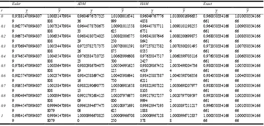
Figure 1 below shows the performance of each method along with the exact solution. Table 1 below shows the solution values for all three methods for 0<r<1. Table 2 below shows the error for all 3 methods.
[image:8.595.162.435.235.411.2]Figure 1. Comparison among the 3 approximate solutions
Table 1. The approximate and exact solution values for 0<r<1
Euler ADM HAM Exact
r
0 0,95881470984807 9 1,00831470984 808 0,9604976737325 36 1,01000016541 999 0,96049767776 4858 1,0100001696635 1 0,960050334166 661 1,010050334166 66
0.1 0,96277470984807 9 1,00732470984 808 0,9644578730675 33 1,00901011558 625 0,96445787711 6751 1,0090101198255 4 0,964050334166 661 1,009050334166 66
0.2 0,96673470984807 9 1,00633470984 808 0,9684180724025 29 1,00802006575 250 0,96841807646 8642 1,0080200699875 6 0,968050334166 661 1,008050334166 66
0.3 0,97069470984807 9 1,00534470984 808 0,9723782717375 26 1,00703001591 875 0,97237827582 0535 1,0070300201495 9 0,972050334166 661 1,007050334166 66
0.4 0,97465470984807 9 1,00435470984 808 0,9763384710725 23 1,00603996608 500 0,97633847517 2427 1,0060399703116 2 0,976050334166 661 1,006050334166 66
0.5 0,97861470984807 9 1,00336470984 808 0,9802986704075 19 1,00504991625 125 0,98029867452 4319 1,0050499204736 4 0,980050334166 661 1,005050334166 66
0.6 0,98257470984807 9 1,00237470984 808 0,9842588697425 16 1,00405986641 750 0,98425887387 6211 1,0040598706356 7 0,984050334166 661 1,004050334166 66
0.7 0,98653470984807 9 1,00138470984 808 0,9882190690775 13 1,00306981658 375 0,98821907322 8103 1,0030698207977 0 0,988050334166 661 1,003050334166 66
0.8 0,99049470984807 9 1,00039470984 808 0,9921792684125 09 1,00207976675 000 0,99217927257 9994 1,0020797709597 2 0,992050334166 661 1,002050334166 66
0.9 0,99445470984807 9 0,99940470984 8079 0,9961394677475 06 1,00108971691 625 0,99613947193 1888 1,0010897211217 5 0,996050334166 661 1,001050334166 66
1 0,99841470984807 9 0,99841470984 8079 1,0000996670825 0 1,00009966708 250 1,00009967128 378 1,0000996712837 8 1,000050334166 66 1,000050334166 66
Table 2. The error for all 3 methods
Euler ADM HAM
_error _error _error _error _error _error
0,0000228471890251404 0,0000312656227772756 0,000000852629996577922 0,0000000108925601114895 0,000000852652340537162 0,0000000108925122404276
[image:8.595.37.563.453.705.2]results. According to the experimental results obtained, we can say that all three methods are giving close solution values with relatively small errors.
REFERENCES
Abbasbandy, S. 2006. Homotopy perturbation method for quadratic Riccati differential equation and comparison with Adomian's decomposition method, Appl. Math. Comput. 172, 485-490.
Abbasbandy, S. and Allahviranloo, T., Numerical solution of fuzzy differential equation, Mathematical & Computational Applications, Vol.7 No.1, 41-52, 2002.
Abu Arqub, O. 2013. Series solution of fuzzy differential equations under strongly generalized differentiability, Journal of
Advanced Research in Applied Mathematics, 5, 31-52.
Abu Arqub, O., A. El-Ajou, S. Momani and N. Shawagfeh. 2013. Analytical Solutions of Fuzzy Initial Value Problems by HAM,
Appl. Math. Inf. Sci., 7, No. 5, 1903-1919.
Adomian, G. 1989. Nonlinear stochastic systems and application to physics, Kluwer, Dordecht.
Adomian, G. 1990. A review of the decomposition method and some results for nonlinear equations, Math. Compute Model., 7 (13), 17–43.
Allahviranloo, T., S. Abbasbandy, N. Ahmady, E. Ahmady, 2009. Improved predictor-corrector method for solving fuzzy initial value problems, Information Sciences, 179, 945-955.
Babolian, E. H. Sadeghi, Sh. Javadi, 2004. Numerically solution of fuzzy differential equations by Adomian method, 149, 547– 557.
Bede, B. S. G. Gal, 2005. Generalizations of the differentiability of fuzzy number value functions with applications to fuzzy differential equations, Fuzzy Sets and Systems, 151, 581-599.
Ch. Palligkinis, S., G. Papageorgiou, I. 2009. Th. Famelis, Runge- Kutta methods for fuzzy differential equations, Applied
Mathematics and Computation, 209, 97-105.
Dubois, D. H. Prade, 1982. Towards fuzzy differential calculus: Part3, differentiation, Fuzzy Sets and Systems 8, 225-233.
Ebadian, A. F. Farahrooz, A. A. Khajehnasiri, 2017. Homotopy analysis method for the solution of fuzzy fractional telegraph equation by using Laplace transform, Konuralp Journal of Mathematics, 5(1) pp. 193-200.
Effati, S. and Pakdaman, M. 2010. Artificial neural network approach for solving fuzzy differential equations, Information
Sciences, 180, 1434-1457.
Goetschel, R. Voxman, W. 1986. Elementary fuzzy calculus, Fuzzy Sets and Systems, 18, 31-43. Kaleva, O. 1987. Fuzzy differential equations, Fuzzy Sets and Systems, 24, 301-317.
Liao, S. J. 1992. The proposed homotopy analysis technique for the solution of nonlinear problems, Ph.D. Thesis, Shanghai Jiao Tong University.
Liao, S. J. 1995. An approximate solution technique which does not depend upon small parametres: a special example, Int. J.
Nonlinear Mech 30, 371-380.
Liao, S. J. 1997. An approximate solution technique which does not depend upon small parametres (Part 2): an application in fluid mechanics, Int. J. Nonlinear Mech., 32 (1997) 815-822.
Liao, S. J. 2009. Notes on the homotopy analysis method: some definitions and theorems, Commun. Nonlinear Sci. Numer. Simul.
14, 983-997.
Ma, M., Friedman, M. Kandel, A. 1999. “Numerical solutions of fuzzy differential equations”, Fuzzy sets and Systems, 105, 133-138.
Madhuri, 2012. Linear Fractional Time Minimizing Transportation Problem with Impurities, Information Sciences Letters, 1, 7-19.
Otadi, M., M. Mosleh, 2016. Solution of fuzzy differential equations, Int. J. Industrial Mathematics, Vol. 8, No. 1, 73-80.
Rabie, F. Ismail, F. A. Ahmadian, and S. Salahshour, 2013. Numerical Solution of Second-Order Fuzzy Differential Equation Using Improved Runge-Kutta Nystrom Method, 1-11.
Seikkala, S. 1987. On the fuzzy initial value problem, Fuzzy Sets and Systems, 24(3), 319–330.
Shokri, J. 2007. Applied Mathematical Sciences, Numerical Solution of Fuzzy Differential Equations., 1(45), 2231 – 2246.
![Table 2 shows error estimation for different values of r ∈ [0, 1] and h.](https://thumb-us.123doks.com/thumbv2/123dok_us/8891035.950729/6.595.38.549.197.732/table-shows-error-estimation-different-values-r-h.webp)