Hydrol. Earth Syst. Sci., 12, 769–796, 2008 www.hydrol-earth-syst-sci.net/12/769/2008/ © Author(s) 2008. This work is distributed under the Creative Commons Attribution 3.0 License.
Hydrology and
Earth System
Sciences
Which spatial discretization for distributed hydrological models?
Proposition of a methodology and illustration for medium to
large-scale catchments
J. Dehotin and I. Braud
Cemagref Lyon, Research Unit Hydrology and Hydraulics, 3bis Quai Chauveau, CP 220, 69336 Lyon C´edex 9, France Received: 12 January 2007 – Published in Hydrol. Earth Syst. Sci. Discuss.: 10 April 2007
Revised: 18 January 2008 – Accepted: 24 April 2008 – Published: 23 May 2008
Abstract. Distributed hydrological models are valuable tools to derive distributed estimation of water balance components or to study the impact of land-use or climate change on water resources and water quality. In these models, the choice of an appropriate spatial discretization is a crucial issue. It is obviously linked to the available data, their spatial resolution and the dominant hydrological processes. For a given catch-ment and a given data set, the “optimal” spatial discretiza-tion should be adapted to the modelling objectives, as the latter determine the dominant hydrological processes consid-ered in the modelling. For small catchments, landscape het-erogeneity can be represented explicitly, whereas for large catchments such fine representation is not feasible and sim-plification is needed. The question is thus: is it possible to design a flexible methodology to represent landscape hetero-geneity efficiently, according to the problem to be solved? This methodology should allow a controlled and objective trade-off between available data, the scale of the dominant water cycle components and the modelling objectives.
In this paper, we propose a general methodology for such catchment discretization. It is based on the use of nested dis-cretizations. The first level of discretization is composed of the sub-catchments, organised by the river network topology. The sub-catchment variability can be described using a sec-ond level of discretizations, which is called hydro-landscape units. This level of discretization is only performed if it is consistent with the modelling objectives, the active hydro-logical processes and data availability. The hydro-landscapes take into account different geophysical factors such as topog-raphy, land-use, pedology, but also suitable hydrological dis-continuities such as ditches, hedges, dams, etc. For
numeri-Correspondence to: J. Dehotin ([email protected])
cal reasons these hydro-landscapes can be further subdivided into smaller elements that will constitute the modelling units (third level of discretization).
1 Introduction
The growing of concerns about environmental, climate change issues, and the emergence of the concept of sustain-able development, has modified the requirements towards hy-drological modelling. The focus was first on the prediction of the water stream flow at a few locations. The demand has now moved to the prediction of the water balance compo-nents (rainfall, runoff, water storage, transpiration, evapora-tion, groundwater levels etc.) at every point within a catch-ment. The consideration of land-use and human-induced modifications of landscapes is a major concern for water management problems (quantity and quality) such as flood forecasting, the study of the impact of land use evolution on stream flow, pollutants or sediments transport. For some of these questions, the knowledge of the water balance compo-nents is not sufficient and fluxes throughout the landscape are required as well as a proper handling of water pathways. For such questions, a representation of the land-surface hetero-geneities is necessary. In this context, distributed models can be valuable tools as they have the ability to take the landscape heterogeneity into account, and provide distributed output variables. They can be used to test different functioning hy-potheses from which simplified and/or predictive models can be derived for more operational purposes. If reliable output variables are expected, distributed model parameters can be estimated a priori from available information. Verification of these models behaviour can be performed not only on the stream flow at the outlet, but also at intermediate stations and on other variables leading to a multi-objective verification (e.g. Mroczkowski et al., 1997; Beldring, 2002; Engeland et al., 2006; Varado et al., 2006a). There was high expectation about the ability of distributed models to take into account changes in the landscape, especially thanks to the increasing availability of high-resolution information. For small catch-ments, landscape features such as agricultural fields, build-ings, and hedges can be represented explicitly, as well as the water pathways between them (e.g. Moussa et al., 2002; Car-luer and De Marsily, 2004; Branger, 2007). For larger catch-ments, a fine representation is not feasible and simplification is necessary. In this case, the specification of all needed pa-rameters, with a suitable resolution, remains a difficult and uncertain task. As a consequence, some distributed param-eters are often calibrated in practice. Thus the usefulness of such distributed models has been questioned many times due to problems of over-parameterization, parameter estima-tion and validaestima-tion limitaestima-tions (e.g. Beven and Binley, 1992; Grayson et al., 1992a, b; Beven, 2001).
The parameter specification in distributed models is par-ticularly uncertain for large catchments. It depends on the choice of a proper level of discretization to handle the land-scape heterogeneity. This choice should take into account the goals of the modelling and the dominant hydrological pro-cesses. The question is thus: is it possible to design a flex-ible methodology to represent landscape heterogeneity
effi-ciently, according to the problem to be solved? This method-ology should allow a controlled and objective trade-off be-tween available data and the scale of the dominant water cy-cle components. The result should also be a function of the catchment under study and of its specificities, especially its size. The problem of scales and scaling in hydrology, as re-viewed by Bl¨oschl and Sivapalan (1995), is underlying all these questions. These questions also form part of a chal-lenge proposed by various hydrologists (e.g., Beven, 2002a; Reggiani and Schellenkens, 2003) and have led to an active field of research in the framework of the Predictions in Un-gauged Basins (PUB) decade, initiated by the IAHS (e.g., Sivapalan, 2003).
In this paper, we propose a methodology for catchment discretization based on the use of nested discretizations. The first level is composed of a hierarchy of sub-catchments, or-ganised by the river network topology. If consistent with the objectives, the sub-catchment variability can be described using a second level of nested discretizations, composed of “homogeneous” landscape areas within the sub-catchments. This discretization is called hydro-landscape units (Winter, 2001). The hydro-landscapes take into account different geo-physical factors such as topography, land-use, pedology, but also possibly hydrological discontinuities such as ditches, hedges, dams, etc. For numerical reasons these hydro-landscapes can be further subdivided into smaller elements that will constitute the modelling units (third level of dis-cretization).
In the first part, the paper presents a review about this spa-tial discretization and the representation of land surface het-erogeneity within distributed hydrological models. We used this synthesis to derive the principles of our general method-ology. The second part of the paper (Sect. 3) focuses on the second level of discretization and the derivation of hydro-landscape units for medium to large scale catchments. We propose the use of landscape classification techniques to de-fine homogeneous hydrological areas. The objective is to provide rationale for the improvement of land surface het-erogeneity description based on various GIS layers. Tra-ditional GIS layers overlay, can lead to a very fragmented discretization, and to smoothing by using re-sampling tech-niques. These techniques often suppress smaller units, which can have an important role in hydrology. An illustration of the whole discretization method, using data from the Saˆone catchment (11 700 km2)in France, is proposed in Sect. 4. A comparison with traditional methods for the definition of ho-mogeneous areas is also performed in Sect. 4, with a dis-cussion of the interest and limitations of the approach. Sec-tion 5 provides illustraSec-tions on how the principles of spatial discretization, outlined in the paper, are being used to an-swer several questions, and the corresponding models which are being built. Conclusions and perspectives are given in the last section.
J. Dehotin and I. Braud: Variability of input data 771 2 Land surface discretization for distributed
hydrologi-cal models: an overview
The definition of an appropriate spatial discretization for hy-drological models will result from a trade-off between vari-ous, sometimes opposing considerations:
1. What is the objective of the distributed hydrological modelling?
2. Which output variables are required and at which spatial and temporal resolution?
3. What are the measured data and at which resolution are they available?
4. What are the active/dominant hydrological processes on this catchment and what are their functional scales? 5. Which representation of hydrological processes is
rele-vant and at which scale?
6. Which degree of heterogeneity is acceptable within the hydro-landscape units?
We first review these various items. In a second step we use this review as a basis for the proposition of a general methodology for the representation of landscape heterogene-ity in distributed hydrological models, using several levels of nested discretizations.
2.1 What is the objective of the distributed hydrological modelling?
This question might seem trivial but is often not always well defined by the modellers. Refsgaard et al. (2005) retained it as one of the first item in the list of tasks they identified for performing a modelling study while respecting some qual-ity insurance criteria. Examples of possible modelling ob-jectives are: determination of the components of the water balance of a catchment, quantification of flood or draught risk, evaluation of mitigation solutions for the limitation of the river pollution at a given location, test of functioning hy-potheses, and search for dominant hydrological processes. For each objective and a given catchment, the required spa-tial discretization should be different.
2.2 Which output variables are required and at which spa-tial and temporal resolution?
The definition of the objective of the study leads to the def-inition of the output variables of interest, and of the spatial and temporal resolution at which they are required or rele-vant. For water balance analysis, the outputs are the various components such as runoff, evapotranspiration, groundwa-ter recharge, wagroundwa-ter storage etc. For pollutant transfer prob-lems, outputs can be, integrated fluxes, maximum concen-trations over a given time step, durations over which legal
thresholds are exceeded. These outputs can be required at annual, monthly, daily, hourly time scale; at distributed loca-tions within sub-catchments or only at the outlet of the whole catchment. A general rule is that a coarser resolution in time and space for output data requires a coarser representation of surface heterogeneity. But there is no clear rule to define that appropriate resolution.
2.3 What are the measured data and at which resolution are they available?
The measured data includes input forcing variables (rain-fall and climate forcing, but also possibly data about water management, such as irrigation or reservoir operation), out-put variables for verification such as stream flow, soil mois-ture, groundwater levels, surface fluxes, and landscape de-scriptors such as land use, geology, elevation, which are used for model parameter estimation and definition of the hydro-landscape and/or modelling meshes.
When speaking about observations, Bl¨oschl and Sivapalan (1995) distinguish between:
1. The extent of the data, i.e. the zone other which the data set is collected
2. The support of the observation i.e. the spatial resolution at which data are integrated
3. The spacing i.e. the distance in time and space between different observations points.
In this paper, we focus on the spatial resolution, but the tem-poral resolution is obviously linked (e.g. Sko¨ıen and Bl¨oschl, 2006). For modelling purposes, all input data, parame-ters and the verification data are required over the hydro-landscape and/or modelling meshes. Unfortunately, there is often a mismatch between the observations data resolution and the modelling meshes resolution. The support of in-situ measurements is often local. Therefore spatial interpo-lation using techniques such as kriging is required to derive the values over the modelling meshes. Stream flow data are directly integrated over catchment areas and are more con-sistent with the modelling scale, but the number of gaug-ing stations is often much smaller than the number of mod-elled sub-catchments. New measurements techniques such as scintillometers provide a certain space averaging for sensible and/or latent heat flux along transects (Green et al., 2001), but do not yet provide values over sub-catchments.
obvious. Thus the fundamental question “which data resolu-tion is needed for landscape descripresolu-tion to represent hydro-logical processes?” remains open (Puech, 2002). Further-more, remote sensing measurements are often not directly related to the hydrologic quantity of interest. The sensors often only sample the first centimetres of the continental sur-faces, whereas information on deeper soil layers would be required. Multi-disciplinary research amongst hydrologists (and more generally with researchers in environment) and remote sensing specialists is still needed to progress on these questions.
There is also a paradox in this progress of remote sens-ing. Whereas the continental surface can be described with more and more accuracy, even at the scale of a building, the knowledge of the sub-soil is not progressing so rapidly. For example, there is a lack of knowledge on soil proper-ties. The data support is local, spacing and extent are limited due to the difficulty and cost of soil sampling. To derive reliable maps at larger scales, hypotheses about soil organ-isation, forming factors are required. In pedology sophis-ticated classification techniques using geostatistics or fuzzy rules are developed for mapping soil units, but the result re-main uncertain (e.g. Burrough et al., 1997; Lagacherie et al., 1997, 2001). Available data in soil databases often provides rather descriptive information on the soils. Their content is often found disappointing, if not useless by hydrologists who are looking for transfer coefficients. The initiative of Lin et al. (2006) to promote hydropedology as a synergetic disci-pline between hydrologists and pedologists is promising (e.g. D’Herbes and Valentin, 1997), but will require some years to be fruitful. This is under way in Europe where the extension of the HOST (Hydrology of Soil Types initiative, Boorman et al., 1995) classification, derived for UKs, is being tested at the European Union level (Schneider et al., 2007). Progress is also expected on soil characterization with the use of geo-physical techniques, but their use is still limited and they can-not be deployed routinely yet. Therefore, for a while, we will have to cope with the paucity of information related to the soil and sub-soil, while performing hydrological modelling. This fact should not be forgotten when combining these data with the detailed data derived from remote sensing of conti-nental surfaces.
From this analysis of data in hydrology, it is obvious that the information is often not available with the desired accu-racy. Therefore there is a need to revisit modelling objectives according to the available data. The formulation of hydrolog-ical processes and the representation of surface heterogeneity will also be affected, especially if the resolutions of the vari-ous sources of information are different.
2.4 What are the active/dominant hydrological processes on a catchment and what are their functional scales? A lot of former distributed hydrological models were based on Hortonian scheme for the runoff. In such models, the
catchment was subdivided into so-called isochrones surfaces. The hydrograph separation with isotopic techniques showed later that this mechanism was uncommon in some environ-ments (Crouzet, Hubert et al., 1970, cited by Gineste, 1997). In such cases, the hydrograph is mainly composed with the waters present in the soil before the rainy event (Gr´esillon, 1994). This convinces hydrologists of the complexity across scale of flow generation processes inside a catchment.
Lots of research has been dedicated to the determina-tion of hydrological processes characteristic scales. One of the recent examples is provide by Sko¨ıen et al. (2003) and Sko¨ıen and Bl¨oschl (2006) who analysed rainfall, stream flow, groundwater level and soil moisture records from Aus-tria and Australia, using geostatistical tools. They were able to determine characteristic time and scales of respectively one day and one month for rainfall and runoff. They also showed that groundwater levels were not stationary. In space, they found that rainfall was almost fractal without character-istic scales whereas runoff appeared non-stationary but not fractal. This data analysis provided evidence of the consis-tency of the Bl¨oschl and Sivapalan (1995) scale diagram. The latter provides guidance for the definition of appropriate spa-tial and temporal discretizations of the various hydrological processes that are included into a particular model.
However, the range of scales for a given process is still large and the dominant processes can change with scale. This is especially evident for the rainfall-runoff relationship for which various authors have shown a decrease of the runoff coefficient with increasing catchment scale for various hy-drologic and climatic contexts (e.g., Bergkamp, 1998; Braud et al., 2001; Cerdan et al., 2004). A downward approach of model complexity (Klemes, 1983), based on data analy-sis can help in the formulation of a conceptual model of the rainfall-runoff relationship, leading to a parsimonious model using parameters derived from available data. This concept has been recently applied by Jothityangkoon et al. (2001) and Eder et al. (2003) for a semi-arid and an alpine catch-ment respectively. They propose models of the rainfall-runoff relationships at the annual, monthly and daily time scale, by progressively increasing the model complexity un-til a good reproduction of the data behaviour was obtained. The two cases studies show that, according to climate and catchment characteristics, very different models can emerge, with different dominant hydrological processes in both cases. Macropores, preferential flow, re-infiltration, variability of land cover, the influence of micro-topography leading to the concentration of runoff into small channels, are some of the factors being able to explain threshold effects and the ob-served differences in dominant hydrological processes across scales (e.g. Bergkamp, 1998; Lehmann et al., 2006; Sidle, 2006; Zehe et al., 2005).
Several concepts have been proposed to describe and ex-plain the variability of landscape characteristics such as or-ganization, hierarchy or fractal behaviour, leading to the def-inition of various characteristic scales (e.g. Vogel and Roth,
J. Dehotin and I. Braud: Variability of input data 773 2003; Lin et al., 2006). The choice of the dominant
pro-cesses that are represented within the model should help in the choice of the proper level of organisation to keep for the spatial discretization.
2.5 Which representation of hydrological processes is rele-vant and at which scale?
The representation of a process within a model implies the choice of two complementary elements. The first one is the resolution for the spatial discretization and the second one is the process conceptualisation. If we borrow the vocabulary from the atmospherical community, the choice of the reso-lution for the spatial discretization will allow the separation between the processes which are represented explicitly (i.e. for which a prognostic variable with an evolution equation is defined) and the processes which are not described explic-itly and which will be parameterised1(i.e. for which simpli-fied representations are adopted and added to the prognostic equations). According to the resolution chosen for the spatial discretization, some processes can be represented explicitly or parameterised. The adoption of the same vocabulary in hydrology could avoid quarrels on the nature of conceptual or physically based modelling. A process would be concep-tual (or parameterised) at one resolution and physically based (explicitly resolved) at another resolution. In atmospheric sciences, the relative homogeneity of the atmosphere allows a straightforward relation between the choice of the spatial resolution (the resolution of the grid) and the processes that are explicitly resolved. It is thus quite easy to change the method used for process representation according to the spa-tial scale. In hydrology, the picture is more complicated due to the hierarchical nature of the hydrological network and the landscape heterogeneity. The definition of the spatial scale at which explicit representation is required is not straightfor-ward. It could be viewed as a level of organisation which would distinguish between processes which are explicitly re-solved and those which are not. Examples taken from soil description can be found in Vogel and Roth (2003) and Lin et al. (2006). The proper level of spatial discretization could be chosen between geological layers, pedo-landscapes, soil profiles, soil horizons and at smaller scales macropores and soil matrix. Ideally, each level of discretization should cor-respond with a different process conceptualisation. The dif-ficulty of defining a proper level of discretization has led to the proposition of several types of regular and irregular dis-cretizations, as well as to various processes conceptualisa-tions.
For process conceptualisation, plot scale studies al-lowed the derivation of physical equations, extensively used in hydrology such as the Richards equation for sat-1In this context, the word “parameterization” should not be con-founded with the estimation of parameters for which it is often used in hydrology. It would be equivalent to conceptualisation in the hy-drology jargon.
urated/unsaturated water flow, the Boussinesq equation for 2D groundwater flow, the Saint-Venant equation for river or overland flow. At this scale, several parameters in these equations such as the retention curve, the hydraulic conduc-tivity or the surface roughness can be estimated from mea-surements. When using coarse resolutions, it is often as-sumed that the form of the equation remains valid. Then it is necessary to derive so-called effective parameters at those scales (e.g. Bl¨oschl and Sivapalan, 1995). For this purpose the aggregation-disaggregation modelling (Bl¨oschl and Siva-palan, 1995) approach to identify the functional relationship at a larger scale from results at smaller scales can be used (see an example in Viney and Sivapalan, 2004). The down-ward approach of model complexity presented in Sect. 2.4 provides another method to address process conceptualisa-tion at various scales.
Concerning the spatial discretization, several distributed hydrological models are based on a regular mesh over which point scale laws are extended and where effective values of the parameters must be determined. Examples are MIKE-SHE (Abbott et al., 1986a, b), ECOMAG (Motovilov et al., 1999), and TOPKAPI (Ciarapica and Todini, 2002). Some authors contest this approach, referred to as a “reduction-ist” approach (e.g. Gottschalk et al., 2001), arguing that the equation becomes a parameterisation of the process, since parameters cannot be estimated from field measurements (e.g. Beven, 2002b). The choice of the grid size is not al-ways rationalised taking into account the processes that are represented, but seems rather the result of commodity and data resolution. One exception can be found in Beldring et al. (1999) and Motovilov et al. (1999) using the ECOMAG model in the framework of the NOPEX project. They deter-mined the size of the mesh from analysis of averaging prop-erties of point groundwater and soil moisture measurements obtained using a dedicated sampling strategy with nested spacing. Of course, data required for such a study are sel-dom available.
is used in TOPMODEL (Beven and Kirby, 1992). In order to represent land-use heterogeneity, some authors have intro-duced the concept of Hydrological Response Units (HRUs) (e.g., Fl¨ugel, 1995), used in the Soil Water Assessment Tool (SWAT) model (Neitsch et al., 2005). HRUs represent a sub-catchment scale discretization composed of a unique com-bination of land cover, soil and land management. One of the drawbacks is that the HRUs mapping induces merging of smaller units into larger ones by applying smoothing filters. From a hydrological point of view, it may result in a loss of information, as some major hydrological processes can be localised on very small units. Illustrations are re-infiltration of runoff at the bottom of hill slopes in the Sahel (Seguis et al., 2002); runoff decrease due to hedge networks (Viaud et al., 2005).
Another example of hydrological spatial discretization is the concept of Representative Elementary Area (REA) pro-posed by Wood et al. (1988), looking for characteristic spa-tial scales, beyond which the geographical locations of fea-tures could be neglected and the distribution taken into ac-count using statistical distributions. Fan and Bras (1995) questioned the universality of the concept, especially be-cause flow routines and the hierarchical structure of the river network were not taken into account in the analy-sis. This drawback is overcome with the concept of Repre-sentative Elementary Watershed (REWs) proposed by Reg-giani et al. (1998, 1999, 2000) and extended by Tian et al. (2006). In terms of spatial discretization, the term REW is strictly equivalent to the term sub-catchment. But Reg-giani et al. (1998, 1999) have proposed a unifying theory for the modelling of hydrological processes on these spa-tial entities. In their approach, REWs form the elementary modelling units divided into several zones corresponding to the various hydrological processes. Global mass, momentum and energy balance laws are formulated at the sub-catchment scale. The corresponding equations remain unchanged what-ever the scale (e.g. for REWs defined at various Strahler or-der). On the other hand fluxes between REWs and their zones (saturated, non-saturated, overland, concentrated and river flow) must be defined for each scale. Sub-catchment variability can be parameterised in the derivation of these fluxes. The strength of the approach is therefore to translate the general problem of model formulation into the problem of derivation of closure relationships at various scales (Reg-giani and Schellekens, 2003). Lee et al. (2005), Reg(Reg-giani and Rientjes (2005) or Zhang et al. (2005) have provided vari-ous formulations of these closure relationships, but further work is still needed to develop closure relationships that ade-quately represent the effect of within-REW heterogeneity on REW fluxes. As an illustration, Varado et al. (2006a) on a case study in Benin, have shown that it could be important to describe sub-catchment scale heterogeneity, especially in the unsaturated zone, in order to get results consistent with mea-surements of stream flow and groundwater levels. Therefore there is a need to combine the various approaches, retaining
the strength of each one, in order to get a spatial discretiza-tion consistent with the characteristic scales and dynamics of the various processes.
2.6 Consequences for the definition of modelling units and process representation: a practical proposition for catchments discretization
The picture drawn from the review of the various items above might result quite confusing. As mentioned above, contrary to atmospheric sciences, it’s difficult to define a unique scale separating processes being represented explicitly from those that must be parameterised. It’s due to the hierarchical na-ture of the river network and the landscape complexity across scales. Furthermore characteristic scales are different for the various processes. Therefore we propose to adopt an approach suggested by Leavesley et al. (2002). It requires that, for a given catchment and a given problem, we replace the question “which model is most appropriate for a specific set of criteria?” by the following one “what combination of process conceptualisations is most appropriate?”. This ap-proach is consistent with the downward apap-proach mentioned previously and the recognition of the “uniqueness of place” as stated by Beven (2003). It also allows building a specific model for a specific objective, taking into account the avail-ability of data. This pleads for the use of multi-scale hydro-logical framework, where the processes are develop as inde-pendent components, using the facilities provided by Object Oriented Modelling and, if possible with their characteris-tic time and space scales. They are then coupled through adequate tools provided by the modelling environment (for recent reviews about environmental computing frameworks, see for instance Argent, 2004; Krause et al., 2005).
The work presented in this paper forms part of a more gen-eral effort aiming at developing such a modelling framework, using an improved description of the landscape heterogene-ity for distributed hydrological models. In order to represent landscape heterogeneity efficiently according to the mod-elling goals, we propose a flexible methodology for catch-ment discretization, based on nested discretizations (Fig. 1). i) The first level is composed of the hierarchy of sub-catchments, linked by the river network topology.
ii) If consistent with the modelling objectives, the active hydrological processes and data availability, sub-catchment variability can be refined using a second level of discretiza-tion: the hydro-landscapes units. They allow refining the es-timation of exchange fluxes within the subcatchment. The discretization can take into account different geophysical factors such as topography, land-use, geology, pedology, but also hydrological discontinuities such as ditches and hedges, etc., in order to represent sub-catchment variabil-ity, consistently with the characteristic spatial and tempo-ral scales of the represented hydrological processes. The hydro-landscapes units can also be discretized vertically into
J. Dehotin and I. Braud: Variability of input data 775
Fig. 1
Fig. 2
Fig. 1. Flow diagram of the three-level discretization procedure.
cells to take into account the vertical structure of soil profiles (Haverkamp et al., 2004).
iii) Finally, if required by the process conceptualisation and/or numerical considerations such as convexity require-ment, a third discretization level can be used and the hydro-landscapes can be subdivided into smaller elements, the modelling units. Note that heterogeneity within hydro-landscapes can be taken into account in a statistical way us-ing for instance the “tile” approach (e.g. Koster and Suarez, 1992) used in atmospheric sciences, if the geographical lo-cation of these heterogeneity is not important. Conservation laws can be solved on the obtained elementary volumes, with various degrees of complexity.
The first discretization level (sub-catchments) is per-formed, using traditional terrain analysis, based on the Dig-ital Elevation Model. This level is not detailed in this pa-per (for more details see Dehotin, 2007). The second dis-cretization level (hydro-landscape) requires the used of dif-ferent kinds of landscape data. The available data needed to describe the landscape heterogeneity inside the model are characterized by different spatial resolutions. In addition, we need to define hydro-landscape consistently with the char-acteristic spatial and temporal scales of the represented hy-drological processes. In the next section we focus on this second level discretization and introduce a method providing rationales for the determination of hydro-landscapes units across scales. The third discretization level can be required according to numerical constraints associated with the meth-ods used to represent hydrological processes. We present an illustration of the third discretization level in section 4.
3 Subdividing catchments into hydro-landscapes: a practical proposition
3.1 Principle of the hydro-landscape delineation
As mentioned in Sect. 1, for small catchments, landscape fea-tures such as agricultural fields, buildings, and hedges can be represented explicitly, as well as the water pathways between them. We can even end up with standard partial differential equations. The conservation laws can be solved using appro-priate numerical methods, which are consistent with the ex-change fluxes approach. At larger scales, such a representa-tion is not feasible and simplified representarepresenta-tions are needed. In the remaining of the section we focus on the second level of discretization and introduce a method providing rationales for the determination of hydro-landscapes units for medium to large catchments. The principle of hydro-landscape is de-scribed in Fig. 2. The first step consists in the definition of homogeneous areas using the data set available. In a second step, the homogeneous areas map is combined with the first level discretization map (sub-catchments), and with other vector maps required to represent hydrological processes to end up with the final hydro-landscape delineation.
Fig. 1
Fig. 2
Fig. 2. Flow diagram of hydro-landscape delineation.
any confidence about the final homogeneous zones map. In the remaining of the section, we present a methodology to derive homogeneous zones for medium to large catchments, based on classification techniques.
3.2 Subdividing medium to large catchments in homoge-neous zones: classification requirements
Hydro-landscapes, introduced by Winter (2001), can be de-fined as areas where hydrological processes can be consid-ered as homogeneous. They can be considconsid-ered as an exten-sion of the HRU concept or of the Representative Elementary Columns – RECs – proposed by Haverkamp et al. (2004). Their delineation can take into account what will be referred to as factors below, influencing hydrological processes, e.g. slope, land use, geology, pedology, etc. The choice of the retained factors depends on the modelling goal, and the con-sidered hydrological processes.
In general, the map obtained by the overlay of various GIS layers leads to a very fragmented picture (see Fig. 7d for ex-ample), which is not necessarily consistent with the variabil-ity of hydrological processes. For hydrological modelling this variability needs to be simplified. Traditional meth-ods are based on smoothing techniques, which suppress the smallest units using area thresholds for instance. The re-sults do not take into account the underlying hydrological processes, whereas the role of these small units can be very important. Improvements are therefore needed to end up with a more rational methodology. The discretization methodol-ogy should remain flexible enough to fit with objectives con-cerning the consistency of scales and the simplification of the patterns. Therefore, the method should allow a better control on the errors arising from the overlay of maps at different resolutions, in an objective and quantifiable way.
As a practical solution, we suggest to extend the princi-ple of landscape classification, used is soil mapping for the definition of homogeneous areas. It allows defining differ-ent levels of complexity in landscape represdiffer-entation that can be associated with different levels of accuracy in hydrolog-ical processes description. The parameters used in the clas-sification can be adapted to the dominant hydrological pro-cesses and the resolution of the final units remains consistent with the resolution of the available data. We borrowed the principles of our landscape classification from those used in soil mapping (Burrough et al., 1997) and more specifically from the method of Masson (1994, 1995); Robbez-Masson et al. (1999); Lagacherie et al. (2001). The latter is based on the definition of reference zones and an analysis of the neighbourhood composition at each location.
3.3 Homogeneous areas delineation principles using clas-sification technique
The different steps of the homogeneous areas delineation method are the following:
1. Identification of the available data and their resolution. Various maps describing several catchment characteris-tics can be used as factors (slope, soil, lithology, land-use...). The classification is a raster-based method. Thus all maps must be in a raster format and are re-sampled with the same resolution, usually the finer one. Note that the procedure could stop here if the data are not sufficient to fulfil the objectives.
2. Choice of relevant hydrological processes and their rep-resentation according to the available data.
J. Dehotin and I. Braud: Variability of input data 777 3. Definition of thepfactors expected to be influential on
these hydrological processes, according to the chosen representation.
4. Simplification of each factor into np classes. This is especially relevant for continuous data such as slope. Then thep factors maps are overlaid using GIS. This overlay leads to a map of the combined factors com-posed of a maximum of
P
Q
j=1
njcombined factors. One class is therefore a unique combination of the p fac-tors. Up to this step, the procedure is therefore similar to the classical GIS layers overlay used for instance in the HRU approach.
5. Definition of the reference zones on the study catch-ment. They are areas associated with a unique com-bination of the retained factors, which can be related to a specific hydrological response, for instance a zone prone to saturated excess runoff.
6. Choice of a neighbouring window (size and shape) and of a descriptor of the composition of the combined fac-tors within this neighbourhood. The neighbourhood window allows to relate each pixel to the pixels inside this window and thus to take into account its surround-ing pixels to perform the classification. A descriptor of the pixels distribution within the neighbouring win-dow is used to characterize each point (pixel) in the landscape. The reference zones are characterized using the same descriptor of the combined factors within each zone.
7. Mapping of the whole catchment using a pixel-by-pixel analysis. Each pixel is allocated to one of the refer-ence zones according to a distance criterion between the descriptor of its neighbouring window composition and that of the reference zones.
8. Estimation of the distance map, which can be consid-ered as a confidence map of the classification.
9. Iteration from steps 6 to 8 until a resolution ensuring a given accuracy and consistency with the input data is obtained. This step is important since the accuracy of the final map depends on the size of the neighbourhood window. Accuracy can be inferred using the confidence map.
We present an illustration of the whole methodology in section 4 and will now detail steps 3 to 9 in Sects. 3.4 to 3.6. 3.4 Definition of landscape factors (step 3 to 4)
In natural sciences, there is not a unique definition of a “land-scape” amongst disciplines. In agriculture, agro-landscape refers to an ensemble of fields that are classified according
to natural vegetation, wooded zones, river network, topogra-phy and soil surface characteristics (Girard, 2000). In soil sciences, pedology is considered as the results of several in-teracting factors (climate, geology, slope, land use), which are used to define soil-landscapes. In ecology, eco-regions are defined as land and water extends including distinct nat-ural community.
For hydrology, the factors that will be retained in the anal-ysis will depend on the modelled hydrological processes. To model infiltration, factors such as soil surface characteristics, soil types, management practices will be influential. To sim-ulate runoff, we can consider topography, topographical in-dex, and soil surface characteristics. For evapotranspiration modelling, land-use, orientation, groundwater levels (geol-ogy), snow melt (topography, orientation) can be taken into account. Once all needed factors are identified, their corre-sponding layers/maps superposition using GIS gives a com-posed picture of the landscape. This comcom-posed picture de-fines various combinations of the landscape factors charac-terizing the spatial organization and characteristics of water dynamics within the sub-catchment.
3.5 Definition of references zones (step 5)
Fig. 3
Fig. 4
Fig. 5
Fig. 3. Illustration of the neighbourhood window’s definition.
If there is a good knowledge of the catchment, the refer-ence zones can be quite easily defined and delineated using the a priori knowledge of field hydrologists. The latter can know the location of areas prone to saturation, or with high slopes, etc. For larger catchments or catchments where it is not possible to perform intensive field surveys, the task is more difficult. In this case, only the factors map can provide the available information. These maps can be used to define possible reference zones, according to traditional/standard knowledge about hydrological processes. In this case, a sim-plified classification of factors can be used and the reference zones can be defined using a statistical and spatial analysis of the multivariate map (see details in Sect. 4). The relevance of such delineation can then be confirmed by a specific field survey.
3.6 Mapping of homogeneous zones (steps 6 to 9)
3.6.1 Neighbourhood definition and characterization of all point in the catchment (step 6)
“Landscape is what is around you” (Robbez-Masson, Foltˆete et al., 1999). With this sentence these authors argue that the integration of spatial neighbourhood is necessary to de-scribe the landscape. With this mapping approach, each point in the landscape is characterized by the composition of a neighbourhood window around the point (contextual anal-ysis). The modeller must define the size and the shape of a neighbourhood window (e.g. ellipsis neighbourhood window on Fig. 3). The latter determines the resolution of the final units. All points in the catchment are characterized using the composition of their neighbourhood window.
The characterization of each point is performed (inside the neighbourhood window) using a descriptor on the multivari-ate image (in pixels). The descriptor may be a histogram, a mean or a standard deviation. This descriptor is calculated for each of the points of the multivariate image. In the
ex-ample provided in the left of Fig. 4, each colour of the pixels characterizes a specific combination of factors and we chose the histogram as a descriptor. To derive it we consider all the pixels inside the neighbourhood window (here a square) and count the number of each combination class (i.e. each colour) in this window. This histogram is constructed for each point of the map.
The choice of the shape of the window allows taking into account some anisotropy in the catchment. For instance ellip-sis neighbourhood window with the major axe oriented north south can be chosen if specific factor (e.g. topography) has such an orientation.
3.6.2 References zones characterization and mapping pro-cedure (steps 6 to 9)
Similarly for each point of the map the references zones are characterized by their composition, using the same descrip-tor, according to the combination factor map (right of Fig. 4). The mapping consists of assigning all points in the land-scape the most similar reference zone in a statistical sense. Similarity is defined as the minimization of the distance be-tween the descriptor of each characterized point and those of the references zones. The distance may be the modal dis-tance, Kolmogorov distance or Manhattan distance (Robbez-Masson, 1994). See the illustration of the principles in Fig. 4. The result of the mapping consists in two maps. The first map represents a segmentation of the initial multivariate im-age into elementary landscape units or polygons. This map is thus composed of homogeneous and unstructured areas. The second map can be considered as a confidence map for the classification. This map represents the distance between the descriptor (e.g. histogram) of each point and the affected reference zone descriptor (e.g. histogram). It quantifies the reliability of the modelling units by providing a criterion of the statistical quality of the classification. If the confidence map is not satisfactory, the classification can be improved by adding more reference zones to get a better representation of the landscape.
3.6.3 Scale and accuracy assessment (step 9)
The size of the hydro-landscapes in the final map depends of the size of the neighbourhood window. This size must be chosen in consistency with the resolution of the input data. The size of the smallest units on the classified map cannot be lower than the finest units of the input maps. An itera-tive procedure is therefore needed to define a neighbourhood window size, consistent with this first constraint. This itera-tive procedure consists in testing several sizes for the neigh-bourhood window until the constraint is fulfilled (iteration of steps 6 to 8). This ensures consistency of the modelling units with the input data resolutions.
Once the “optimal” size of the neighbourhood windows is chosen, the classification can be improved using the distance
J. Dehotin and I. Braud: Variability of input data Fig. 3 779
Fig. 4
Fig. 5
Fig. 4. Basic principles for the mapping by landscape classification. On the left map is figured a point to be mapped (the black one) with
a squared neighbourhood window and the composition histogram within this window. On the right map are shown the reference zones and their composition histograms. In the middle the Manhattan distance is used to search for the minimum distance between the left histogram and those of the reference zones.
map. The latter provides an idea of the accuracy of the clas-sification. If the distance is large, it means that the similarity of the neighbourhood with the available reference zones is poor. Therefore, new references zones can be added in the areas with larger distances and used to improve the mapping (iteration of steps 6, 7 to 9). This will reduce uncertainties on the landscape heterogeneity representation and handling. 3.7 Determination of the hydro-landscapes and modelling
meshes
As shown in Fig. 2, the hydro-landscapes are obtained by overlaying the map of homogeneous areas and the sub-catchments map. Other vector maps can be added at this stage. These maps may describe hydrological discontinu-ities, or specific boundary maps, that are important for the modelling. After this step, the discretization result consists of irregular polygons composing an unstructured mesh. Ac-cording to the numerical method used for the representa-tion of some processes, these meshes can be directly used as modelling units (e.g. vertical infiltration with one dimen-sional Richard’s equations, or evaporation flux simulation). In some other cases, such as the resolution of partial differ-ential equations using the finite volumes or finite elements method, these meshes cannot be directly used, because they are not convex. A third level of discretization is thus needed. This third level of discretization consists in deriving con-vexes meshes based on the hydro-landscapes of the second level of discretization. This can be obtained by forcing the hydro-landscapes polygons with Triangular Irregular Net-works (TINs) or by using specific algorithms to derive con-vex meshes from the hydro-landscapes.
Fig. 5. Location of the upper-Saˆone catchment in France.
In the next section, we present an illustration of the whole methodology through the detailed presentation of a case study. For the determination of homogeneous areas, we also present a comparison with more traditional approaches. The goal of the comparison is to show which method produces the “best” representation of the landscape heterogeneity. The comparison through hydrological model results is beyond the scope of the paper and will be reported in other publications.
4 Illustration of the methodology using data from the upper-Saˆone catchment in France
France (Fig. 5). The river rises in the Vosges Mountains in Lorraine, and flows south through Burgundy. The ele-vation ranges from 177 a.m.s.l. at the outlet to more than 1215 a.m.s.l. in the Vosges. The main land-use classes are broad-leaved forests, arable land, and pastures. The arable land is mainly located in the south-western part, whereas the pastures are located in the north-eastern part of the catch-ment. The forests are spread all over the catchment and in the Vosges, coniferous forest is important. Urban surfaces constitute about 2% of the catchment area with the largest concentration around the town of Dijon. The geology is char-acterised by limestone in the southern parts and sandstones and granites in the northern parts.
We first present the available data and their resolution, as well as the objectives of the study. Then, we illustrate the nested discretization procedure of Fig. 1. For the definition of homogeneous areas, all the steps outlined in Sect. 3 are presented. The results of the classification are also compared with traditional procedures.
4.1 Available data and objectives of the modelling The available data for this catchment include:
– 3 h time resolution values of precipitation (rain and snow), potential evapotranspiration, and the maximum and minimum temperatures, distributed on 8×8 km grid for the period 01/08/1981–31/07/1998 and provided by M´et´eo-France.
– Daily stream flow data from the French hydrographic database (Banque Hydro) for the period 01/08/1981– 31/07/1998 at 22 gauging stations. Their catchment areas cover a wide spectrum ranging from 52 to 11 700 km2.
– A digital elevation model (DEM) with resolution 200 m, 100 m and 1000 m from the IGN (Institut G´eographique National) in France and provided by Water Agency (Agence de l’eau).
– The Corine Land Cover database provided by Institut Franc¸ais de l’ENvironnement (IFEN) with a 500 m res-olution. The database contains 44 land cover classes organized in three levels (Bossard et al., 2000).
– A soil map from the Soil information system of France from National Institute of Agronomic Research (INRA) with a 1/1 000 000 resolution (Jamagne et al., 1995). For about one-third of the catchment, another soil database at 1/250 000 resolution was available from the IGCS (Inventaire Gestion et Conservation des Sols) lead by INRA (http://www.gissol.fr/ or http://www.igcs-stb. org/)
– The geology map of France with a 1/1 000 000 resolu-tion from the BRGM (Bureau de Recherche G´eologique et Mini`eres).
– A referential of groundwater systems from SANDRE specification (Secr´etariat d’Administration Nationale des Donn´ees Relatives `a l’Eau) and available at the web site http://sandre.eaufrance.fr/.
We can underline the large heterogeneity in the resolution of input maps. Furthermore, meteorological data, which deter-mine the hydrological response, provide the coarser informa-tion, both in space and in time. These data are not used in the definition of the hydro-landscapes units, but the information should be taken into account in the choice of the processes representation and then in the final discretization.
As shown in Fig. 1, the first step is to define the modelling objectives. The goal of our study is to evaluate the impact on the water cycle, of changes in the land-use. The target vari-ables are the water balance components at the daily, monthly and annual time scales and for sub-catchments with a min-imum size of about 50 km2 (the size of the smallest catch-ment where stream flow data is available, but also the order of magnitude for the meteorological data mesh). The following processes are considered: evapotranspiration, water transfer within the non-saturated and saturated zones, and river flow. No detailed representation of runoff is considered. Further details on the choice of the methods for the representation are given in Sect. 5.1.
With these modelling objectives in mind, we used the var-ious sources of information as follows for the spatial dis-cretization of the catchment. First we used the DEM to extract the river network and delineate the sub-catchments (first discretization level, Sect. 4.2.1). For the determination of hydro-landscape units (second level of discretization and sub-catchment scale variability) we used the lithology, land use and slope maps (Sect. 4.2.2.), soil map and the ground-water referential. If required by the process representation and numerical constraints, further sub-divisions of hydro-landscape units can be performed (third level of discretiza-tion). For instance, hydro-landscape can be subdivided to get convex polygons for the application of finite volumes meth-ods.
4.2 Catchment discretization for a distributed water bal-ance components derivation
The first step in the discretization is to determine the sub-catchments (Sect. 4.2.1). A large degree of heterogene-ity, especially in land-use, is still present within each sub-catchment. We assume that it must be taken into account for an accurate simulation of evapotranspiration and this justifies the determination of hydro-landscapes units and the use of a second level of discretization. The relevance of this choice should of course be proven through simulation, but it is be-yond the scope of the paper, where we only wish to illus-trate our methodology for landscape discretization, using the available data of the upper-Saˆone catchment.
J. Dehotin and I. Braud: Variability of input data 781
Fig. 6 :
Fig. 7
Fig. 6. Discretization of the catchment in sub-catchments using the first (a) and second (b) Strahler order.
4.2.1 A first discretization into sub-catchments
The first discretization level was that of the sub-catchments. Sub-catchments were determined using DEM analysis and river network structure. Several algorithms were proposed to extract hydrological information from DEM (Peuker and Douglas, 1975; Martz and Garbrecht, 1992). We used the Tardem algorithm (Tarboton, 1997) to derive sub-catchments from the 200 m resolution DEM. The 200 m resolution DEM can be used because the modelling does not include a fine representation of runoff. The algorithm we used first per-formed a detection and treatment of depression zones in the DEM. Then the local direction of out-flows were calculated for each cell using the D8 algorithm. The contributing areas were determined for each cell in terms of drained area and a threshold area was used to define river cells. We used a vec-tor file of the actual river network provided by the National Geographic Institute (France). The TARDEM algorithm al-lows to enforce the drainage direction to follow an existing river network (using DEM correction). In this case, the au-tomatic network extracted from the DEM is the same as the existing river network used to force the drainage direction. The sub-basins drained by every link of the river network were delineated using a threshold for the Strahler order of the river links. Figure 6a and b show a discretization of the Saˆone catchment in sub-catchments using the first and sec-ond Strahler orders. The number of sub-catchments was 341 and 81 for the first and second order respectively, with an average area of 35 and 147 km2 respectively. These values were quite large but related to the fact that the existing net-work only considered permanent river reaches.
Table 1. Table defining the factors and the delimitation of classes
for the whole classification.
Land Use Urban areas Open spaces Agricultural areas Vineyards and fruit trees Pastures
782 J. Dehotin and I. Braud: Variability of input data
Fig. 6 :
Fig. 7
Fig. 7. Maps of (a) land-use, (b) slope and (c) lithology on the upper Saˆone catchment. (d) Map of the combination of the three previous
factors. Superimposed is the discretization of the catchments into sub-catchments at the two Strahler order.
4.2.2 Catchment discretization into hydro-landscapes
Because of the catchment’s size, the available data and the modelling goal presented in Sect. 4.1, the hydro-landscape delineation requires the mapping of homogeneous areas (Fig. 2). In this section, we performed the homogeneous areas delineation using the method proposed in Sect. 3.3. Delineation of the homogeneous zones
Factors definition and data selection
The modelling objective was the determination of the distributed components of the water balance at various time scales. One of these components is evapotranspiration and we considered land-use as one of its controlling factors. We assumed that the partition of incoming rainfall between runoff and infiltration was controlled by factor such as lithology and slope. Other factors such as the topographic index of Beven and Kirkby (1979), as well as the direct use of soil-landscape units could have been considered. In the
example described below, we therefore considered three factors: lithology, slope and land-use. The next step was to simplify the information through the definition of classes for continuous data such as slope. In the case of the Saˆone, we reclassified the original 26 classes of the Corine Land cover map (resolution: 500 m), present in the catchment, into nine classes, especially because the distinction of the various urban areas was not useful for the study. This classification was corresponding to expected differences in hydrological response, especially evapotranspiration. In the same way we simplified the lithology map according to the parent material and the age of the layers, leading to seven classes for lithology (scale: 1/1 000 000). The slope map was derived from the DEM analysis discussed in Sect. 4.1 and classified into five classes (resolution: 200 m). The various classes for the different factors are given in Table 1. All the maps were re-sampled with a 200 m resolution and were used to define the map of combined factors. The maps of factors are shown in Fig. 7a, b and c. Figure 7d shows the multivariable image of the combined factors obtained after superposition of the three data layers. It is composed of 221
J. Dehotin and I. Braud: Variability of input data 783 classes of combined factors (amongst the 9×5×7=315
pos-sible classes) and formed the basis for the hydro-landscape mapping procedure. Figure 7d shows that the variability of these factors is large within a sub-catchment. It is an argument for considering this second level of discretization. Definition of the references zones
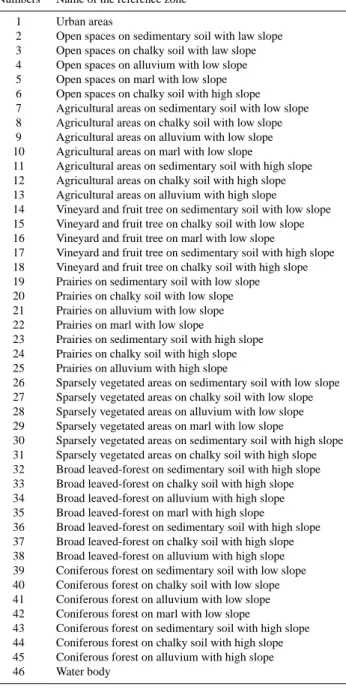
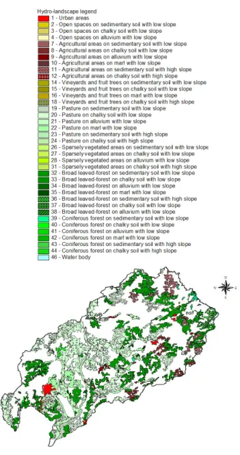
The definition of reference zones may be the most dif-ficult step of this approach. In an ideal case, reference zones should result from a good knowledge on the catchment (e.g. Peschke et al., 1999 for the definition of factors controlling infiltration excess and saturation excess areas). Usually, this is not the case, as for the upper-Saˆone catchment. Therefore, we chose to define references zones using spatial analysis of a simplified combination of landscape factors. This map was derived using the 9 classes for land-use, 2 classes for slopes (low and high) and 4 classes for lithology (see Table 1). They were used to define 46 types of reference zones (Table 2). Their location is shown in Fig. 8 and was defined by ensuring the representativeness of each reference zone in all areas over the catchment. As much as possible, we chose areas with a certain degree of homogeneity. Mapping procedure
For the mapping procedure, we used an available soft-ware named CLAPAS developed by Robbez-Masson (1994) (http://www.umr-lisah.fr/Produits/Clapas/). It allows map-ping using landscape classification techniques. Several descriptors of the neighbourhood are available: mean, standard deviation, histogram, and matrix of co-occurrence. The software proposes several choices of the neighbourhood window shape: square, ellipse, circle, ring etc. The squared neighbourhood window is usually used. We used a square, as particular anisotropy handling was not needed. The histogram of composition was used as descriptor (of neigh-bourhood window and references zones) and the Manhattan distance to compute the similarity with the composition of the reference zones. The choice of the Manhattan distance is justified since it is more robust than the other distances (Kolmogorov, Cramer, etc.) used for performing similarity between vectors (Robbez-Masson, 1994).
Each point X within the catchment was characterized by a specific histogram of the possible combined factors (p=221) within the neighbourhood window, denoted by
MX=(d1, d2, . . ., dp). The histogram calculation was also performed for eachk=46 references zones. For a reference zone j, the histogram is noted Mj=(m1j, m2j, . . ., mpj). Affectation of a point X to a reference zone j consists of minimizing the Manhattan distanced(Mx, Mj)calculated by Eq. (1); see Fig. 4:
Table 2. Table defining the reference zones type.
Numbers Name of the reference zone 1 Urban areas
2 Open spaces on sedimentary soil with law slope 3 Open spaces on chalky soil with law slope 4 Open spaces on alluvium with low slope 5 Open spaces on marl with low slope 6 Open spaces on chalky soil with high slope 7 Agricultural areas on sedimentary soil with low slope 8 Agricultural areas on chalky soil with low slope 9 Agricultural areas on alluvium with low slope 10 Agricultural areas on marl with low slope
11 Agricultural areas on sedimentary soil with high slope 12 Agricultural areas on chalky soil with high slope 13 Agricultural areas on alluvium with high slope
14 Vineyard and fruit tree on sedimentary soil with low slope 15 Vineyard and fruit tree on chalky soil with low slope 16 Vineyard and fruit tree on marl with low slope
17 Vineyard and fruit tree on sedimentary soil with high slope 18 Vineyard and fruit tree on chalky soil with high slope 19 Prairies on sedimentary soil with low slope 20 Prairies on chalky soil with low slope 21 Prairies on alluvium with low slope 22 Prairies on marl with low slope
23 Prairies on sedimentary soil with high slope 24 Prairies on chalky soil with high slope 25 Prairies on alluvium with high slope
26 Sparsely vegetated areas on sedimentary soil with low slope 27 Sparsely vegetated areas on chalky soil with low slope 28 Sparsely vegetated areas on alluvium with low slope 29 Sparsely vegetated areas on marl with low slope
30 Sparsely vegetated areas on sedimentary soil with high slope 31 Sparsely vegetated areas on chalky soil with high slope 32 Broad leaved-forest on sedimentary soil with high slope 33 Broad leaved-forest on chalky soil with high slope 34 Broad leaved-forest on alluvium with high slope 35 Broad leaved-forest on marl with high slope
36 Broad leaved-forest on sedimentary soil with high slope 37 Broad leaved-forest on chalky soil with high slope 38 Broad leaved-forest on alluvium with high slope 39 Coniferous forest on sedimentary soil with low slope 40 Coniferous forest on chalky soil with low slope 41 Coniferous forest on alluvium with low slope 42 Coniferous forest on marl with low slope
43 Coniferous forest on sedimentary soil with high slope 44 Coniferous forest on chalky soil with high slope 45 Coniferous forest on alluvium with high slope 46 Water body
d(MX, Mj)= p
X
i=1
di−mij
(1)
Fig. 8
Fig. 8. Map of the reference zones.
Resulting hydro-landscapes and distance maps
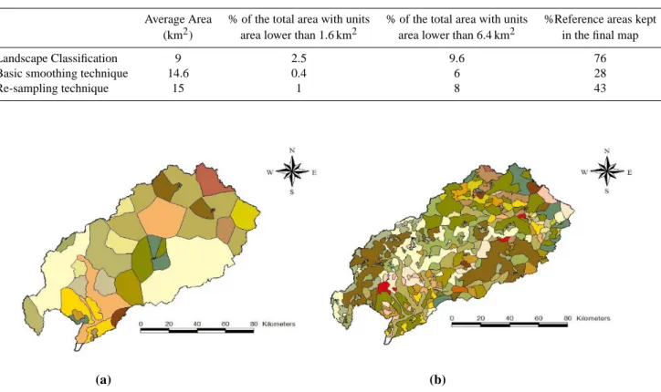
In the first iteration, we used a neighbourhood win-dows resolution of 3 km. In a second iteration, we tried to refine the mapping by using a smaller neighbourhood window of 2.2 km. In a third step, we tested a window’s size of 1.4 km. Figure 9 shows the maps of the hydro-landscapes and their corresponding distance maps for three sizes of the neighbourhood window: 3, 2.2 and 1.4 km. In Fig. 9 (right), the yellow colour corresponds to pixels that are correctly classified (i.e. with a low value of the Manhattan distance) whereas the blue colour corresponds to pixel which are badly classified (high values of the Manhattan distance). Figure 10 shows the distribution of the area of the mapped units and Table 3 provides the corresponding statistics. Table 3 shows
that the average area of the map units dropped when the neighbourhood window decreased. When the neighbour-hood window decreased, the map units were smaller, and the number of coarse features decreased. On Fig. 9 (right), we can see that the decrease of the neighbourhood window was leading to an improvement of the confidence map (less blue colour).
Choice of the mapping that fits well with the input data
The use of different sizes for the neighbourhood win-dows provided modelling units at different resolutions. The statistical analysis of the area distribution provided a way to assess the consistency of the results with the resolutions of the input data. The finest scale of the input data was 1/250 000 and the coarser scale was 1/1 000 000. The final modelling unit could not be more accurate than the finest scale. For a scale of the classified map of 1/250 000, the rule of “quart” states that the modelling units must have an area larger than 1/4th of 2.5×2.5 km2, i.e. 1.6 km2. For a scale of the classified map of 1/1 000 000, the units should be larger than 1/4th of 10×10 km2, i.e. 6.4 km2. The percentage of the cumulated areas occupied by the units with area lower than these two thresholds are provided in Table 3.
A trade off is needed to choose the most appropriate map. The first one (top of Fig. 9) with an average area of 16 km2 seemed too coarse compared to the resolution of the input data. In the third map (bottom of Fig. 9) the average area of 5 km2is consistent with a scale of 1/250 000 for the classified map. However this feeling of accuracy may be misleading because 18 % of the total area was composed of units with an area smaller than 6.4 km2and about 6% of the total area was composed of units with area smaller than 1.6 km2. The bet-ter compromise may be to choose the second map (middle, Fig. 9) with an average area around 9 km2. More than 90% of the total area was covered with landscape units having an area larger than 6.4 km2and more than 97% of the total area was covered with landscape units having an area larger than 1.6 km2. Thus, the iterative procedure of this classification approach provided an efficient tool to assess the mapping resolution according to the input data resolution. Further-more, the distance map provided an idea of the uncertainties on the modelling units representation, and could be used for uncertainty analysis. The final choice of the window size res-olution can also be conditioned by sources of information, not taken into account in the classification procedure. For instance, in the case of the Saˆone catchment, the input rain-fall was available on square grids of 64 km2. Therefore, the first map resolution (Fig. 9, top left) could be more consistent with rainfall resolution for hydrological modelling.
Other modelling objectives and/or other factors map res-olution would produce different maps. We performed addi-tional simulation to test the sensitivity of homogeneous zone mapping to the chosen factors. The mapping criteria were
J. Dehotin and I. Braud: Variability of input data 785
Table 3. Statistics of the areas of the mapped units for several sizes of the neighbourhood window.
Average area Standard deviation % of the total area with units % of the total area with units (km2) of area (km2) area lower than 1.6 km2 area lower than 6.4 km2
Map 1 (3 km) 16 99 1 5
Map 2 (2.2 km) 9 70 2.5 9.6
Map 3 (1.4 km) 5 34 6 18.4
Fig. 9a
Fig. 9b
Fig. 9b. Left: hydro-landscapes units and Right: distance map for the neighbourhood window of 2.2 km.
the same as those used for the middle map of Fig. 9. The reference zones were the same; the neighbourhood windows shape and size were also the same. The results (Fig. 10, left) were compared with the Fig. 9 (middle) map, (redrawn in Fig. 10, right). We performed two kinds of tests. In the first test, we replaced the slope map by the topographic in-dex map. The result (Fig. 10a) shows that two new reference landscapes appeared: “Pasture on chalky soil” and “Agricul-tural areas on high slope”. On the other hand, the “Broad leaved-forest on chalky soil” disappeared. In the second test, the topographic index was added to the factors used for the mapping of Fig. 9 (slope, lithology, and land use). The result
(Fig. 10c) shows that the “Pasture on chalky soil” and the “Broad leaved-forest on chalky soil” were well represented in the final map. This example illustrates that, the choice of the factors retained in the analysis really influence the ho-mogeneous zone mapping. The presented technique allows a large flexibility in landscape heterogeneity representation. It is likely to ensure a relevant representation of heterogeneity according to the available data (factors) and modelling ob-jectives.
J. Dehotin and I. Braud: Variability of input data 787
Fig. 9c
Fig. 9c. Left: hydro-landscapes units and Right: distance map for the neighbourhood window of 1.4 km.
Comparison with the usual mapping techniques for homoge-neous areas delineation
In this section, we present the results of two traditional mapping techniques to delineate homogeneous areas and compare them with those of the classification methodology presented before. Traditional mapping techniques are based on area threshold criteria. For the usual mapping techniques we used areas threshold criteria of 6.4 km2 and 1.6 km2 corresponding respectively to the minimum and maximum scale of input data. Exhaustive evaluation of the
classifica-tion methodology needs a comparison for a range of models, but we focus at this stage on the capacity of the method to represent efficiently landscape heterogeneity. We show that the methodology allowed handling in more rational manner the uncertainties of heterogeneity representation in distributed modelling.
Mapping results with the basic smoothing techniques
Fig. 10
Fig. 11
Fig. 10. Comparison between mapping units when using different landscape factors. (a) Factors used: land use, topographic index and
lithology. (c) Factors used: land use, topographic index, slope and lithology. (b, d) reference map units (redraw of Fig. 9 middle).
Fig. 10
Fig. 11
Fig. 11. Fraction of the total area occupied with units landscapes
of area lower than the area given in abscissa for three values of the neighbourhood window.
of the map units. Usually, the basic technique (we used the ArcView smoothing function) consists in removing areas smaller than those representing the resolution of the input data. The corresponding maps are shown in Fig. 12 and the
statistics of the areas of the mapped units can be found in Table 4.
When areas with areas smaller than 6.4 km2 were re-moved, the average area of the map units was of about 255 km2. Less than 0.04% of the total area was mapped with units having an area lower than 6.4 km2 (Fig. 12a). The mapped units were very coarse and the picture was not very satisfactory. When removing areas lower than 1.6 km2 (Fig. 12b), the average area of the units was of about 32 km2 and about 1% of the total area was covered with units having an area lower than 6.4 km2.
Mapping by re-sampling and smoothing technique
The final map of hydro-landscapes can be obtained by re-sampling the original multivariate map (the one shown in Fig. 7d) of the combination of factor in order to get a smoother image. For this re-sampling (we used the resam-pling function of ArcView), only the desired final factors were considered (in our case the 46 factors retained for the reference zones). Then the same smoothing technique as