A framework for assessing flood frequency based on climate projection information

www.hydrol-earth-syst-sci.net/13/2119/2009/ © Author(s) 2009. This work is distributed under the Creative Commons Attribution 3.0 License.

Earth System

Sciences

A framework for assessing flood frequency based on climate

projection information

D. A. Raff1, T. Pruitt2, and L. D. Brekke2

1_{Flood Hydrology and Emergency Management Group, Technical Service Center, Bureau of Reclamation,} Denver, CO 80225, USA

2_{Water Resources Planning and Operations Support Group, Technical Service Center, Bureau of Reclamation,} Denver, CO 80225, USA

Received: 7 February 2009 – Published in Hydrol. Earth Syst. Sci. Discuss.: 9 March 2009 Revised: 22 September 2009 – Accepted: 7 October 2009 – Published: 10 November 2009

Abstract. Flood safety is of the utmost concern for water

resources management agencies charged with operating and maintaining reservoir systems. Risk evaluations guide de-sign of infrastructure alterations or lead to potential changes in operations. Changes in climate may change the risk due to floods and therefore decisions to alter infrastructure with a life span of decades or longer may benefit from the use of climate projections as opposed to use of only historical ob-servations. This manuscript presents a set of methods meant to support flood frequency evaluation based on current down-scaled climate projections and the potential implications of changing flood risk on how evaluations are made. Methods are demonstrated in four case study basins: the Boise River above Lucky Peak Dam, the San Joaquin River above Fri-ant Dam, the James River above Jamestown Dam, and the Gunnison River above Blue Mesa Dam. The analytical de-sign includes three core elements: (1) a rationale for select-ing climate projections to represent available climate pro-jections; (2) generation of runoff projections consistent with climate projections using a process-based hydrologic model and temporal disaggregation of monthly downscaled climate projections into 6-h weather forcings required by the hydro-logic model; and (3) analysis of flood frequency distributions based on runoff projection results. In addition to demonstrat-ing the methodology, this paper also presents method choices under each analytical element, and the resulting implications to how flood frequencies are evaluated. The methods used re-produce the antecedent calibration period well. The approach results in a unidirectional shift in modeled flood magnitudes. The comparison between an expanding retrospective (current

Correspondence to: D. A. Raff

([email protected])

paradigm for flood frequency estimation) and a lookahead flood frequency approach indicate potential for significant bi-ases in flood frequency estimation.

1 Introduction

The design and safety assessment of large dams in the western United States requires estimates of flood frequency. Flood frequency relates the magnitude of floods with their probabilities of occurrence. Often flood frequencies are de-scribed by return period. The return period concept, as of-ten communicated in the community and practice, is that a 100-year flood is an event that should happen, on average, once every hundred years. A more strict interpretation of a flood frequency for a 100-year flood is that it is a flood that is believed to have a probability of being equaled or ex-ceeded of 0.01 in any one year. While we do not wish to challenge the current paradigm of communication of flood hazard, it is reasonable to question the paradigm of what a return period means within a nonstationarity system (Siva-palan and Samuel, 2009). The nonstationarity concern and current paradigm are not mutually exclusive if it is acknowl-edged that a flood with a 100-year return period is not a con-stant value. Or, working within our preferred strict interpre-tation of the flood return period, a flood with an exceedance probability of 0.01 this year may have a different exceedance probability in the future.

climate, and given how flood risks are generated from the observed record of the past, it may be prudent to include in-formation that not only describes the flood potential of the past but also of the future.

Flood frequency estimation within the United States gov-ernment has as its fundamental doctrine, Bulletin 17-B published by the Interagency Advisory Committee on Wa-ter Data (IACWD, 1982). Released in 1982, Bulletin 17-B provides guidance for observational data treatment and parameter estimation for flood frequency distributions (IACWD, 1982). The general methodology of Bulletin 17-B is to gather a time series of annual maximum floods at the lo-cation that the user wishes to determine the flood magnitude versus frequency relationship. In additional to the gage in-formation, any historical information about large floods that may pre-date the gage record is also used. Fundamentally, Bulletin 17-B assumes that flood potential can be described by a three parameter log-Pearson distribution (log-Pearson III distribution). It is known that of the three parameters (mean, standard deviation, and skew) the skew is most sensi-tive to the information set. Bulletin 17-B, therefore, provides guidance on estimating the skew based upon a weighted sum of the collected data set and regional estimates of skew. All of the information is then used to fit to a log-Pearson III pa-rameter distribution1. This fitted distribution then describes the probability of an annual maximum flood being exceeded. The process used in Bulletin 17-B assumes many things such as that the annual maximum floods are independent sam-ples from a general population. This idea that information from the past is a good indication of current potential or fu-ture potential is called a stationarity assumption. This sta-tionarity assumption may be less valid when the climate is changing and the flood potential at a location may be chang-ing along with the climate. Nearly three decades ago it was acknowledged within Bulletin 17-B that little attention was given to the subject of non-stationarity and that future stud-ies were needed. Within Bulletin 17-B, although the word non-stationarity is not used explicitly, the concept is alluded to among the eight recommendations for future studies. It was identified that there is a need to account for watersheds altered by urbanization whose flood potential may not be re-flected by the observed and historical data at the location (p. 27+28, IACWD, 1982).

That vast majority of research since the release of Bulletin 17-B has been focused on improved treatment of historical data from instrumental records and/or historical and pale-oflood proxies. There are studies that have looked at more ef-ficient selection of distributional parameters (e.g., Lane and Cohn 1996, O’Connell et al., 2002, Stedinger et al., 1988) that perform better when compared to Bulletin 17-B (e.g., Cohn et al., 1997; England, 2003). There are studies that 1_{This is a generalization of a more complex procedure that takes} into account, for example, outlier data and consideration for mixed-population flood generation mechanisms.

have improved estimates of uncertainty (e.g., Cohn et al., 2001; O’Connell et al., 2002) and those that avoid a distri-butional assumption (e.g., O’Connell, 2005). These methods have improved the treatment of historical data and as a col-lection have made vast strides forward to fitting distributions to data that has been collected for a specific site when an as-sumption of stationarity is supportable. There has also been work in an attempt to expand our assumptions of known vari-ability through the incorporation of paleoflood data which may have come from a different climate than that observed or known in the historical record (e.g. Frances et al., 1994; O’Connell, 1999).

It is acknowledged that the assumption of historical cli-mate stationarity has always been questionable in flood fre-quency estimation. This assumption would appear to become even more questionable in the future (e.g., Milly et al., 2008), particularly as a warming climate may to lead to changes in precipitation regime, seasonality, and other characteristics relevant to floods. Some studies have focused on how shifts in climate might lead to changes in extreme events such as precipitation and temperature (Manabe et al., 1980; Easter-ling et al., 2000). The Intergovernmental Panel on Climate change recently reported in their fourth assessment report that the climate is warming and that it is very likely that heavy precipitation events will increase in frequency over most areas (IPCC, 2007a). Evidence has been mounting that precipitation rates and patterns have been changing in the ob-servational record (e.g., Alexander et al., 2006; Kunkel et al., 2003; Kanae et al., 2004). There are further studies that have used climate projections to show shifts in future pre-cipitation patterns (e.g., Easterling et al., 2000; Emori et al., 2005). Changes in extreme precipitation patterns have con-sequences for changes in flood patterns. Hamlet and Letten-maier (2007) showed that there were changes in flood risks during observed warming of the 20th century.

There have been process-based approaches to consider changes to floods and flood frequencies. Using GCM pro-jections, Hirabayashi et al. (2008) have simulated daily dis-charges for projected climate and shown changes in precipi-tation and flood patterns that they identified as an increased frequency of flooding over many regions except North Amer-ican and central to western Eurasia. Cameron et al. (2000) used GCM simulations to drive the TOPMODEL hydrology model to show the changes to probability of occurrence of specific discharges for the gauged, upland Wye catchment in Wales, UK. Sivapalan and Samuel (2009) illustrate an ap-proach to use process-based methods to estimate flood fre-quencies that do not rely upon stationarity assumptions for three catchments in Australia.

flood potential into the future. To evaluate the physical re-sponse to a changing climate there remains limited guidance on how to incorporate climate projection data into a frame-work for flood hazard assessment. In this manuscript meth-ods to address this gap in planning capabilities are intro-duced. The methods described are meant to identify whether climate change may influence risk assessments made using Bulletin 17-B. The methods are designed to reveal flood frequency consistent with climate projection information at a user-specified future period. Methods are demonstrated in four case study basins: the Boise River above Lucky Peak Dam, the San Joaquin River above Friant Dam, the James River above Jamestown Dam, and the Gunnison River above Blue Mesa Dam. The analytical design includes three core elements: (1) a rationale for selecting climate pro-jections with the objective of representing the breadth of climate projection information available; (2) generation of runoff projections consistent with climate projections, using a process-based hydrologic model and temporal disaggre-gation of monthly downscaled climate projections into sub-monthly weather forcings required by the hydrologic model; and (3) analysis of flood frequency distributions based on runoff projection results.

2 Data sources and methods

The following methods describe the steps utilized in this manuscript to estimate flood frequency from climate projec-tions. There were four river basins considered (Sect. 2.1). The focus is to evaluate the physical response to climate pro-jections through the use of a hydrologic tool (Sect. 2.2). The general methodology described below is to use GCM projec-tions of temperature and precipitation to drive a hydrology model. The GCM projections are at a spatial and temporal scale incompatible with modeling flood flows so spatial and temporal downscaling methods will be employed.

For each of the four river basins a subset of 9 climate pro-jections of temperature and precipitation were chosen from a candidate pool of 112 potentials at each of three lookahead periods (2011–2040, 2041–2070, and 2071–2099) (Sects. 2.3 and 2.4). For each of the climate projections a weather gen-eration scheme was employed to temporally disaggregate the monthly climate projection values into 6-h values (Sect. 2.5) necessary to drive the hydrologic tool. The weather gen-eration approach has a random component to it and there-fore was applied 10 times per projection. Ten random gen-erations were chosen, somewhat arbitrarily, through assess-ment of the differences among each random generation. The hydrologic simulations result in a set of flows from which the annual maximum discharges were compiled. The sim-ulated annual maximum discharges were then considered in the context of estimating flood risk through flood frequency analyses (Sect. 2.6).

Fig. 1. Basin Selections are the Boise River above Lucky Peak

Dam, the James River above Jamestown Dam, the San Joaquin River above Friant Dam, and the Gunnison River above Blue Mesa Dam.

2.1 Basin selection

The effect of a changing climate may vary geographically. Therefore, to determine the suitability of the methods pro-posed it was desired to have a geographically diverse set of examples. Four geographically diverse reservoir watersheds were considered, each having dams that were either built by the Bureau of Reclamation (BOR) or significantly influence Reclamation operations. The four basins are the Boise River, above Lucky Peak Dam, the James River above Jamestown Dam, the Gunnison River above Blue Mesa Dam, and the San Joaquin River above Friant Dam (Fig. 1). Each of these basins has a strong snowmelt component to flood generation. Most often these basins have annual maximum discharges that are snowmelt only, or rain-on-snowmelt events. It is ex-pected, however, that there are different geographic and other conditions that affect flood response to climate change (Ham-let and Lettenmaier, 2007).

Lucky Peak Dam is located at 43◦₃₁0_{N, 116}◦₀₃0_{W on}

reservoir elevation and forested and subalpine terrain in the higher elevations.

Jamestown Dam is located at 46◦550N, 98◦420W on the James River approximately 1.5 miles from Jamestown, North Dakota. The elevations in the basin range from approxi-mately 450 m at the dam to approxiapproxi-mately 580 m. The wa-tershed area upstream of the dam is approximately 4750 km2 (1750 mi2). The “knob and kettle” drainage area is the re-sult of the most recent glaciation. There are numerous de-pressions, or closed portions, that do not drain or drain in-frequently. The mean annual precipitation over the basin is approximately 480 mm with the majority falling from May to September.

Blue Mesa Dam lies at 38◦₂₇0_{N, 107}◦₂₀0_{W on the}

Gun-nison River near GunGun-nison in south central Colorado. The dam impounds Blue Mesa Reservoir and drains approxi-mately 8900 km2 (3434 mi2). The drainage is some of the most rugged of the entire Colorado River basin consisting of peaks over 4265 m high with long sloping ridges, and nar-row valley floors. The elevation at the dam site is approx-imately 2290 m. Mean annual precipitation varies from ap-proximately 760 mm in the high elevations to apap-proximately 250 mm in the valleys.

Friant Dam is located near 37◦000N, 119◦420W on the San Joaquin River about 19 miles from Fresno, California. The dam impounds Millerton Lake. The drainage area at Fri-ant Dam is approximately 4120 km2(1591 mi2). Drainage is from the western slope of the Sierra Nevada range. Eleva-tions in the basin range from 170 m at the dam to just under 4260 m along the crest of the Sierra Nevada range. The ter-rain in the basin may be described as rugged forest. Mean annual precipitation over the basin is approximately 900 mm which varies significantly by elevation.

2.2 Hydrologic tool

The hydrologic model used in this study is the National Weather Service River Forecast System (NWSRFS) Sacra-mento Soil Moisture Accounting (SAC-SMA) Model (Bur-nash et al., 1971). The SAC-SMA Model is coupled to the Anderson Snow Model of snow accumulation and ablation (Anderson, 1973). This model was chosen because it is the operational model of the National Weather Service and cal-ibrated models for all of the chosen basins were available. SAC-SMA consists of two upper and three lower soil mois-ture storage zones. The two upper zones are free and tension water storage and the three lower zones are a primary free, a supplemental free and a tension water storage zone (Bur-nash, 1995). The snow accumulation and ablation model computes a freezing height to distribute rain and snow by el-evation. The NWSRFS SAC-SMA Model has a long history of operational use within the United States Federal Agencies. Despite the fact that this study looks at characterization of fu-ture climate, calibration sets based on an antecedent period

were not altered for the future period. Further discussion of this assumption can be found in Sect. 3.4.

2.3 Climate projections data

In order to evaluate the potential changes in flood frequency from projected climate changes it is desired to have a current set of climate projections that encapsulate the projected fu-ture climate variability. In preparation for the IPCC’s fourth assessment report (IPCC, 2007a, b), climate model output was collected as the World Climate Research Programme’s (WCRP’s) Coupled Model Intercomparison Project phase 3 (CMIP3) multi-model dataset (Meehl et al., 2007). The CMIP3 archive houses projections made from climate mod-els that include coupled atmospheric and ocean general circu-lation models (GCMs). Each of these models simulate global response to various future greenhouse gas emissions paths (IPCC, 2000). The GHG emission paths were defined begin-ning from the end of the 20th century from lower to higher emission rates of carbon dioxide into the atmosphere as a subjective function of global technological and economic de-velopments during the 21st century.

The grid resolutions of the CMIP3 models are O(102)km, which is not appropriate to evaluate the impacts to local flood hydrology where information at less than O(10) km is needed. For example, the hydrologic models used in this study are used to support operational flood forecasting ob-jectives and have been applied at resolutions of O(10) km to appropriately represent flood-relevant hydrologic processes. Spatial downscaling is used to bridge this gap in spatial res-olution. There are two broad types of downscaling available, dynamic and statistical. A statistical downscaling approach was selected for use here as it provides information that is well tested and documented, automated and efficient enough to permit downscaling of many projections, able to produce output that statistically matches historical observations, and is capable of producing spatially and temporally continuous fine-scale precipitation and temperature information at the basins modeled (Brekke et al., 2009). Potential drawbacks to a statistical downscaling approach include the lack of ca-pability of a statistical approach to identify or model local climate effects and land-surface feedbacks (Salathe et al., 2007). There is a further inherent assumption of stationarity that the statistical relationships observed between fine scale observations of the past and the GCMs are relationships that will continue in the future. Despite these drawbacks the sta-tistical approach has been shown to provide capabilities com-petitive with dynamical methods (Wood et al., 2004). There are multiple methods to accomplish statistical downscaling (e.g., Wood et al., 2002; Wood et al., 2004; Maurer and Hi-dalgo, 2008).

CMIP3 Climate Projections” archive http://gdo-dcp.ucllnl. org/downscaled cmip3 projections/ (Maurer et al., 2007). These data were developed using a statistical downscal-ing technique called bias-correction spatial disaggregation (Wood et al., 2002, 2004) that has been used to support nu-merous investigations on projected hydrologic impacts under climate change (Payne et al., 2004; Van Rheenan et al., 2004; Maurer, 2007; Christensen and Lettenmaier, 2007; Anderson et al., 2008; Brekke et al., 2009). The data archive includes downscaled projections of 112 CMIP3 projections of simu-lated monthly climate from 1950–2099 and at 1/8◦ spatial resolution.

All 112 projections were obtained for the latitude lon-gitude coordinate of the dam for the purposes of projec-tion selecprojec-tion described in Sect. 2.4 and subsequently over the entire basin in support of the weather generation meth-ods described in Sect. 2.5. The particular projections are available at the archive described above. For the pur-pose of numbering the 112 projections they were numbered first by model in ascending alphabetical order, second by emissions path in ascending alphabetical order, and finally by model run in ascending numeric order. For example, the projections are labeled<model>.<path>.<run>in the archive and the projections numbered here #1 through #3 are therefore bccr bcm2 0.1.sresa1b, bccr bcm2 0.1.sresa2, and bccr bcm2 0.1.sresb1, respectively.

2.4 Projection selection

The desire of using projected climate and considering more than a single projection is to portray that there is not a known future climate and to consider the variability with respect to temperature and precipitation changes and lookahead peri-ods. Ideally to estimate flood risk at some point in the fu-ture one could assign a probability distribution to the expec-tation of temperature and precipiexpec-tation. For example one ap-proach could be to use all 112 projections, treated as equally likely as an ensemble representation of projected climates. This approach has the advantage of not requiring assign-ment of probabilities to specific projections. However, the results would tend toward the central tendency of the 112 projections with little weight on the projections that show dramatic shifts and may have the most significant implica-tions on flood risk. A second approach could be to attempt to evaluate model performance over the historical period at the locations of interest and use the “best” models for projec-tions. This approach, however, has been shown to be diffi-cult and sensitive to evaluation metric (Gleckler et al., 2008; Reicher et al., 2008). In addition, it might not reduce the assessed projection uncertainty given the role of emissions scenarios and initialization options in establishing this un-certainty (Brekke et al., 2008).

Here a method was chosen that chose a subset of 9 GCM model projections that encapsulate the variability of precip-itation and temperature. This information, as opposed to

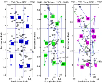
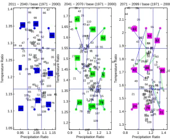
at-tempting to identify a specific risk can be used to show the range of risk that may exist. The selected nine projections are allowed to vary by lookahead period. Three lookahead periods were considered, 2011–2040, 2041–2070, and 2071– 2099. These periods represent three different decision time frames in which one might change operations or physical infrastructure. A tercile grid is constructed based upon the projected temperature and precipitation relative to the simu-lated historical antecedent period (1971–2000) (Fig. 2). The tercile grid is generated through a Cartesian sectioning be-tween the maximum and minimum changes in precipitation and temperature at the lookahead period relative to the an-tecedent period. The GCM projections that were geomet-rically calculated to be closest to the nine vertices encom-passing the array of projected temperature and precipitation shifts were chosen. Projections have internal climate dynam-ics and just as there is observed interdecadal variability in the observed and historical past, the climate models have inter-decadal variability in their projected future. The interinter-decadal variability are not necessarily synchronous with each other and also do not necessarily share the same dynamics or initial conditions and have other differences Projections, therefore, depending when in the future they are examined, may display different relative precipitation and temperature. The relative precipitation and temperature of the 9 selected GCM projec-tions are hence different by lookahead period. In Fig. 2 the blue lines in the second and third panel represent the location of projection from the 2011–2040 lookahead in the 2041– 2070 and 2071–2099 lookahead, respectively. For example, for the Gunnison River above Blue Mesa for the lookahead period of 2011–2040 projection 87 (ncar ccsm3 0.6.sresa1b) represents the GCM projection geometrically closest to the tercile of smallest precipitation ratio and largest temperature ratio Fig. 2 – first panel). At the 2041–2070 lookahead pe-riod projection 87 remains in the upper third of temperature amongst the projections but is in the middle third of precipi-tation ratios. At the 2071–2099 lookahead period, projection 87 is in the middle third of both precipitation and temperature ratios.

2.5 Weather generation

(a) Gunnison River above Blue Mesa Dam

0.9 1 1.1

1.2 1.3 1.4 1.5 1.6 1.7 1.8 1.9 2 1 2 3 4 5 6 7 8 9 10 11 12 13 14 15 16 17 18 19 20 21 22 23 24 25 26 27 28 29 30 31 32 33 34 35 36 37 38 39 40 41 42 43 44 45 46 47 48 49 50 51 52 53 54 55 56 57 58 59 60 61 62 63 64 65 ₆₆ 67 68 6970 71 72 73 74 75 76 77 78 79 80 81 82 83 84 85 86 87 88 89 90 91 92 93 94 95 96 97 98 99 100 101 102 103 104 105 106 107 108 109 110 111 112 Precipitation Ratio Temperature Ratio

2011 − 2040 / base (1971 − 2000)

97 54 63 44 111 22 87 70 76

0.9 1 1.1

1.4 1.6 1.8 2 2.2 2.4 2.6 2.8 1 2 3 4 5 6 7 8 9 10 11 12 13 14 15 16 17 18 19 20 21 22 23 24 25 26 27 28 29 30 ₃₁ 32 33 34 35 36 37 38 39 40 41 42 43 44 45 46 47 48 49 50 51 52 53 54 55 56 57 58 59 60 61 62 63 64 65 66 67 68 69 70 71 72 73 74 75 76 77 78 79 80 81 82 83 8485 86 87 88 89 90 91 92 93 94 95 96 97 98 99 100

101 102 103

104 105 106 ₁₀₇ 108 109 110 111 112 Precipitation Ratio Temperature Ratio

2041 − 2070 / base (1971 − 2000)

36 97 107 92 27 21 46 75 81

0.8 1 1.2

2 2.5 3 3.5 4 1 2 3 4 5 6 7 8 9 10 11 12 13 14 15 16 17 18 19 20 21 22 23 24 25 26 27 28 29 30 31 32 33 34 35 36 37 38 39 40 41 42 43 44 45 46 47 48 49 50 51 52 53 54 55 5657 58 59 60 61 62 63 64 65 66 67 68 69₇₁7072

73 74 75 76 77 78 79 80 81 82 83 84 85 86 87 88 89 90 91 92 93 94 95 96 97 98 99 100 101 102 103 104 105 106 107 108 109 110 111 112 Precipitation Ratio Temperature Ratio

2071 − 2099 / base (1971 − 2000)

62 110 3 26 11 22 43 58 21

(b) San Joaquin River above Friant Dam

0.8 1 1.2

1.02 1.03 1.04 1.05 1.06 1.07 1.08 1.09 1.1 1.11 1.12 1 2 3 4 5 6 7 8 9 10 11 12 13 14 15 16 17 18 19 20 21 22 23 24 25 26 27 28 29 30 3132 33 34 35 36 37 38 39 40 41 42 43 ₄₄ 45 46 47 48 49 50 51 52 53 54 55 56 57 58 59 60 61 62 63 64 65 66 67 68 69 70 71 72 73 74 75 76 77 78 79 80 81 82 83 84 85 86 87 88 89 90 91 92 93 94 95 96 97 98 99 100 101 102103 104 105 106 107 108 109 110 111 112 Precipitation Ratio Temperature Ratio

2011 − 2040 / base (1971 − 2000)

35 39 78 86 29 79 87 27 74

0.8 1 1.2

1.06 1.08 1.1 1.12 1.14 1.16 1.18 1 2 3 4 5 6 7 8 9 10 11 12 13 14 15 16 17 18 19 20 21 22 23 24 25 26 27 28 29 30 31 32 33 34 35 36 37 38 39 40 41 42 43 44 45 46 47 48 49 50 51 52 53 54 55 56 57 58 5960 61 62 63 64 65 66 67 68 69 70 71 72 73 74 75 7677 78 79 80 81 82 83 84 8586 87 ₈₈ 89 90 9192 93 9495 96 97 98 99 100 101 102 ₁₀₃ 104 105 106 107 108 109 110 111 112 Precipitation Ratio Temperature Ratio

2041 − 2070 / base (1971 − 2000)

36 33 73 43 65 76 41 48 71

0.8 1 1.2 1.4

1.08 1.1 1.12 1.14 1.16 1.18 1.2 1.22 1.24 1.26 1.28 1 2 3 4 5 6 78 9 10 11 12 13 14 15 16 17 18 19 20 21 22 23 24 25 26 27 28 29 30 31 32 33 34 35 36 37 38 39 40 41 42 43 44 45 46 47 48 49 50 51 5253 54 55 56 57 58 59 60 61 62 63 64 65 66 67 68 69 70 7172 73 74 75 76 77 78 79 80 81 82 83 84 85 86 87 88 89 90 91 92 93 94 95 96 97 98 99 100 101 102 103 104 105 106 107 108 109 110 111 112 Precipitation Ratio Temperature Ratio

2071 − 2099 / base (1971 − 2000)

38 37 15 51 2 34 92 47 21

Fig. 2. Projection Selection by lookahead period and basin. Numbers represent spread of individual climate projections. Panels moving from

(c) James River above Jamestown Dam

0.95 1 1.05 1.1 1.15 1.05 1.1 1.15 1.2 1.25 1.3 1.35 1.4 1 2 3 4 5 6 7 8 9 10 11 12 13 14 15 16 17 18 19 20 21 22 23 24 25 26 27 28 29 30 31 32 33 34 35 36 37 38 39 40 41 42 43 44 45 46 47 48 49 50 51 52 53 54 55 56 57 58 59 60 61 62 63 64 65 66 67 68 69 70 71 72 73 74 75 76 77 78 79 80 81 82 83 84 85 86 87 88 89 90 91 92 93 94 95 96 97 98 99 100 101 102 103 104 105 106 107 108 109 110 111 112 Precipitation Ratio Temperature Ratio

2011 − 2040 / base (1971 − 2000)

58 31 74 48 23 82 89 2 24

0.9 1 1.1 1.2 1.3

1.2 1.25 1.3 1.35 1.4 1.45 1.5 1.55 1.6 1.65 1.7 1 2 3 4 5 6 7 89 10 11 12 13 14 15 16 17 18 19 20 21 22 23 24 25 26 27 28 29 30 31 32 33 34 3536 37 38 39 40 41 42 43 44 45 46 47 48 49 50 51 52 53 54 55 56 57 58 59 60 61 62 63 64 65 66 67 68 69 70 71 72 73 ₇₄ 75 76 77 78 79 80 81 82 83 84 85 86 87 88 89 90 91 92 93 94 95 96 97 98 99 100 101 102 103 104 105 106 107 108 109 110 111 112 Precipitation Ratio Temperature Ratio

2041 − 2070 / base (1971 − 2000)

52 5 76 86 63 105 41 20 24

0.8 1 1.2 1.4

1.3 1.4 1.5 1.6 1.7 1.8 1.9 2 2.1 1 2 3 4 5 6 7 8 9 10 11 12 13 14 15 16 17 18 19 20 21 22 23 24 25 26 27 28 29 30 31 32 33 34 35 36 37 38 39 40 41 42 43 44 45 46 47 48 49 50 51 52 53 54 55 56 57 58 59 60 61 62 63 64 65 66 67 6869 70 71 72 73 74 75 76 77 78 79 80 81 82 83 84 85 86 87 88 89 90₉₁

92 93 94 95 96 97 98 99 100 101 102 103 104 105106 107 108 109 110 111 112 Precipitation Ratio Temperature Ratio

2071 − 2099 / base (1971 − 2000)

52 60 31 92 86 78 42 47 24

(d) Boise River above Lucky Peak Dam

0.9 1 1.1 1.2

1.04 1.06 1.08 1.1 1.12 1.14 1.16 1.18 1.2 1.22 1.24 1 2 3 4 5 6 7 8 9 10 11 12 13 14 15 16 17 18 19 20 21 22 23 24 25 26 27 28 29 30 31 32 33 34 35 36 37 38 39 40 41 42 43 44 45 46 47 48 49 50 51 52 53 54 55 56 57 58 59 60 61 62 63 64 65 66 6768 69 70 71 72 73 74 75 76 77 78 79 80 81 82 83 84 85 86 87 ₈₈ 89 90 91 92 93 94 95 96 97 98 99 100 101 102 103 104 105 106 107 108 109 110 111 112 Precipitation Ratio Temperature Ratio

2011 − 2040 / base (1971 − 2000)

35 36 108 89 14 82 97 53 109

0.9 1 1.1 1.2

1.1 1.15 1.2 1.25 1.3 1.35 1 2 3 4 5 6 7 8 9 10 11 12 13 14 15 16 17 18 19 20 21 22 23 24 25 26 27 28 29 30 31 32 33 34 35 36 37 38 39 40 41 42 43 44 45 46 47 48 49 50 51 52 53 54 55 56 57 58 59 60 61 62 63 ₆₅ 64

66 67 68 69 70 71 72 73 74 75 76 77 78 79 80 81 82 83 84 85 86 87 88 89 90 91 92 93 9495 96 97 98 99 100 101 102 103 104 105 106 107 108 109 110 111 112 Precipitation Ratio Temperature Ratio

2041 − 2070 / base (1971 − 2000)

39 4 14 46 17 79 53 98 22

1 1.2 1.4

1.2 1.25 1.3 1.35 1.4 1.45 1.5 1.55 1.6 1 2 3 4 5 6 7 8 9 10 11 12 13 14 15 16 17 18 19 20 21 22 23 24 25 26 27 28 29 30 31 ₃₂ 33 34 35 36 37 38 39 40 41 42 43 44 45 46 47 48 49 50 51 52 53 54 55 56 57 58 59 60 61 62 6364 65 66 67 68 69 70 7172 73 74 75 76 77 78 79 80 81 82 83 84 85 86 87 88 89 90 ₉₁ 92 93 94 95 96 97 98 99 100 101 102 103 104 105 106 107 108 109 110 111 112 Precipitation Ratio Temperature Ratio

2071 − 2099 / base (1971 − 2000)

38 11 73 41 59 3 26 88 94

Table 1. Weather generation scenarios (column 2) and their corresponding sampling constraints (columns 2 and 3). The implication of the

sampling constraints for number of random possibilities shown in column 4.

Weather Generation considerations

Sampling Constraint – scaled month must be from same month as projection

Sampling Constraint – Temperature and Precipitation subdivided to limit scaling constant

Result of Sampling Constraint: Number of observed historical months available for selection for a 50 year calibration set 1-sq Yes, Scaled month must come

from same as projected month

No 50

4-sq Yes, Scaled month must come from same as projected month

Yes 12 or 13

8-sq No, scaled month can be any month

Yes 75

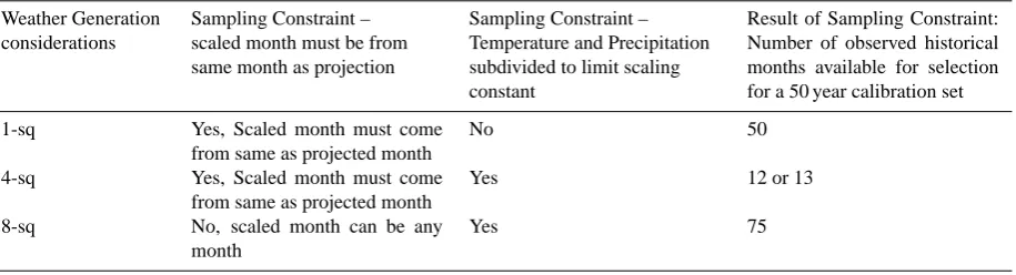
Three separate sampling criteria were considered to create set of 6-hourly values to scale, as described below. All cri-teria preserve the intermittency and timing of storm duration and types that appear within the calibration set. For exam-ple, consider a projection for January 2031 (temperature Jan-uary 2031 = T2031, precipitation JanJan-uary 2031 = P2031) and a set of observed historical Januarys from each SAC-SMA models calibration weather data. A random selection of one of calibration set of January 6-h time series is made, for ex-ample T1990 and P1990. A scale constant is then applied for temperature and precipitation, respectively to the 6-h incre-ments such that the aggregate for both precipitation and tem-perature matches T2031 and P2031 (precip constant * P1990 = P2031, temp constant * T1990 = T2031). The result is a new set of temperature and precipitation values whose mean is consistent with the projection values (2031) but whose tim-ing and intermittency is consistent with the observed values (1990). This choice of methodology is adopted and/or modi-fied from earlier work (Wood et al., 2002). The technique has been used in other hydrologic impacts studies under climate change where monthly climate projections were temporally disaggregated to develop sub-monthly weather forcings (e.g., Payne et al., 2004; Christensen and Lettenmaier, 2007; Mau-rer, 2007).

Key choices in this temporal disaggregation scheme are the eligibility constraints applied to observed-historical months during the process of resampling. Several past im-plementations of this scheme have adopted the constraint that the sampled month only needs to be of the same calendar month as the projected month (denoted “one-square” in this manuscript, or 1-sq for short). With this constraint, it is pos-sible that the projected month may be relatively hot and wet while the resampled observed month is relatively cold and dry. This could lead to rather large scaling ratios applied to the historical month’s 6-h forcings and call into question about whether the new and adjusted forcings are still plau-sible in the context of observed historical data. The tails of flood frequency distributions are important, and this opportu-nity for large scaling ratios can lead to anomalies in the tails

of the distributions. A decision was thus made in this study to consider alternative eligibility constraints on resampling in order to limit such scaling ratios.

Two alternative sampling constraints were considered (Ta-ble 1). The first alternative sampling constraint is called 4-sq (four-square). It involves subdividing the calibration weather years into four categories: hot-wet, hot-dry, cold-wet, and cold-dry. For example for basin A, each January from the calibration set of 1967–1997 were collected and the 6-h observed values were aggregated into monthly mean for temperature and total precipitation. The median temperature amongst these mean monthly values was then found and used to separate hot and cold Januaries. Then for the hot Januaries the median precipitation value was found and the hot Januar-ies were then divided into hot-dry and hot-wet JanuarJanuar-ies. For the cold Januaries the procedure is repeated. The result for the 4 sq method for basin A with 50 years of calibration set data is that there would be 12 or 13 historical Januaries in each of the four categories. Sampling of observed histor-ical months was then constrained so that the categories of sampled and projected months matched in each sampling in-stance. For example if projected January 2031 is hot and dry then the randomly selected 6-h values for scaling must come from the 12 or 13 historical Januaries that have been catego-rized as such.

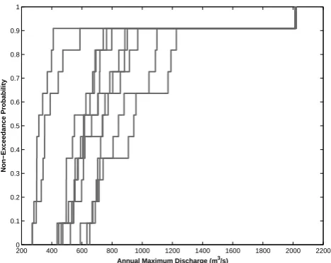
Because there is a random component to the sampling methodology for temporal downscaling it was desired to consider the range of variability that this randomness may induce. Therefore, multiple downscaling simulations were done for each projection selected for each lookahead period. The simulation set size was arbitrarily set to 10 simulations of 6-hourly values to be run through the SAC-SMA hydro-logic model. To show the variability induced through the temporal downscaling methodology consider a single projec-tion. For the lookahead period 2011–2040 there are 30 years of modeled results for each simulation. The key variables of interest for further discussion are the annual maximum floods of each year. For a single projection (inmcm3 0.1.a1b), the temporal downscaling random component results in an em-pirical distribution of the ten simulations that can encom-pass a relatively wide distribution of annual maximum floods (Fig. 3). Empirical cumulative distribution functions of an-nual maximum floods during the lookahead period 2011– 2040 for one projection set are shown in Fig. 3. The 90% non-exceedance level for this projection and simulation set ranges from approximately 400 to 1200 m3/s. The weather generation approach used to generate in Fig. 3 was the 8-sq method.

The National Weather Service considers two methods (sta-tion and area-weighted) for calibrating the SAC-SMA mod-els. The station method involves mapping the gridded GCM data to a location in space using bi-linear interpolation. This method is used if the corresponding SAC-SMA observed mean-area temperature (MAT) for an elevation zone is repre-sented by a “synthetic” station. This is usually the case where there is significant elevation variation across the basin. Ob-served temperature data from a network of climate stations is mapped to the “synthetic” station to produce the MAT for a given basin elevation zone. This “synthetic” station lo-cation is used to extract the GCM gridded data for a given basin elevation zone. The temperature value is interpolated from the four grid cell centers surrounding the “synthetic” station location. Although there is not one single standard for which SAC-SMA models are calibrated an example can be reviewed within Bissell and Orwig (1995).

The area-weighted approach is used in cases where the MAT was developed without the use of a “synthetic” station. This involves intersecting the boundary of the basin elevation zone with the 1/8 degree grid then deriving a temperature value for the zone area by area-weighting the temperature of each grid cell that intersects the zone boundary.

The methods (“sythetic” station vs. MAT) used for cali-bration of the SAC-SMA model by the National Weather Ser-vice were retained when mapping the GCM average tempera-ture data from the 1/8 degree grid to the SAC-SMA basin ele-vation zones. The designation throughout the rest of the anal-ysis is S for station weighting, and AW for area weighting. For example, the weather generation with 8-sq constraints on the Boise River with station weighting is designated S-8sq.

200 400 600 800 1000 1200 1400 1600 1800 2000 2200

0 0.1 0.2 0.3 0.4 0.5 0.6 0.7 0.8 0.9 1

Annual Maximum Discharge (m3_/s)

Non−Exceedance Probability

Fig. 3. Empirical Cumulative Distribution Functions for annual

maximum floods from 1967–1997 retrospective period for in-mcm3 0.1.a1b projection and 10 simulations of 8-sq weather gen-eration.

The James River basin is the only of the four evaluated in this manuscript that had an AW.

2.6 Hydrologic hazard assessment

To put information into a context that is used throughout flood hazard assessment and management the information developed from the simulation model are used to create flood frequency curves. For each projection and each simulation by lookahead there is a modeled annual maximum flood. For each of the three lookahead periods two types of flood fre-quencies were considered, the expanding retrospective flood frequency and the lookahead flood frequency. The expand-ing retrospective is the current paradigm for flood frequency. This is how most flood frequencies are calculated in that all information at a location of interest is considered equally when developing a flood frequency curve. Every year there is a new observation of an annual maximum discharge added to an expanding record of floods at that location. For exam-ple, using expanding retrospective analysis for a basin that has a period of record from 1950–1990 those forty occur-rences of annual maxima would be treated as independent samples from a general population and used to fit a distribu-tion to (i.e. Log-Pearson III from Bulletin 17-B). If time then proceeds to 2020 there would be 30 additional independent samples (i.e., 1950–2020). This approach relies heavily on the stationarity assumption in that all 70 years are assumed to independent samples from the same distribution.

For example, for a location that has a period of record from 1950–2020 as before only the period of 1990–2020 is used to compute the flood frequency. Although the period of 1990– 2020 is considered to be stationary when fitting a distribution it assumes that the period of 1950–1990 does not come from this same distribution.

The expanding retrospective flood frequencies were cal-culated as follows. For the 2011–2040 future period, a total of 60 samples were used to fit the log-Pearson III distribu-tion. These 60 samples comprised 30 random samples taken from between the 5th and 95th quantiles from the length of record of the calibration set for that particular basin and 30 samples taken from the 5th and 95th quantiles between the 2011–2040 simulations. The result is 60 total samples which were then fit to a log-Pearson III distribution as described in Bulletin 17-B without any regional skew adjustment. Be-cause of the random selection of 30 simulations from the 4500 possibilities for the retrospective period and the 30 ran-dom samples from the 2700 possibilities for the 2011–2040 period, the procedure was performed 100 times to account for some of the variability. For the expanding retrospective approach for the 2041–2070 lookahead period, the same pro-cedure was followed as the 2011–2040 period with the ad-ditional 30 random samples taken between the 5th and 95th quantiles from the 30 years by 9 GCM projections by 10 sim-ulations between 2040–2070 for a total of 90 samples. Like-wise there were a total of 120 samples for the 2071–2099 lookahead period.

The lookahead flood frequencies were calculated as fol-lows. For the 2011–2040 lookahead period 30 random sam-ples were taken from between the 5th and 95th quantiles from the 30 years by 9 GCM projections by 10 simulations between 2011 and 2040. The difference between this set and the expanding retrospective set is that for this set there is an absence of the retrospective period. The sample size from which a distribution is being fit is smaller. This is a total of 30 samples which were then fit to a log-Pearson III dis-tribution as described in Bulletin 17-B without any regional skew adjustment. This was repeated 100 times. For the 2041–2070 lookahead period 30 random samples were taken from between the 5th and 95th quantiles from the 30 years by 9 GCM projections by 10 simulations between 2041 and 2070. Again, this is a total of 30 samples which were then fit to a log-Pearson III distribution. The procedure for the 2071– 2099 lookahead was similar. For each of the three lookahead periods using the lookahead flood frequency approach there are 30 years of data from which to fit the log-Pearson III dis-tribution. For the 2071–2099 lookahead period the difference between the lookahead approach (30 years data) and the ex-panding retrospective approach (120 years data) is 90 years of data. The implications of reducing the sample size in an attempt to better characterize the population from which the floods are being observed are examined later in the docu-ment.

3 Results and discussion

3.1 Weather generation for evaluating flood potential

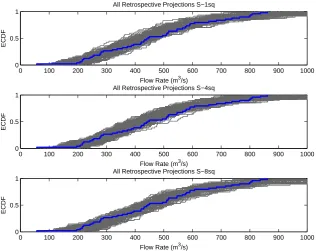
Three sampling constraints (variations) described in Sect. 2.5 were considered from a weather generation method based on historical resampling. It was desired to use only one of the three variations to evaluate changes to flood frequency. A comparison of performance was therefore made between the weather generation variations. The comparison metric cho-sen was the calibration set used for each of the NWSRFS SAC-SMA models. As described in Sect. 2.4 for each of the three lookahead periods there were nine projections se-lected based on their variation in temperature and precipita-tion. With ten simulations available per projection and a fifty year calibration set there are a combined, 13 500 annual max-imum discharges per location over the antecedent period. An evaluation was made to evaluate how many of the simulations and weather generation sequences encapsulated the observed historical annual maximum flows at each basin. It was deter-mined that the 8-sq weather generation constraint variation produced empirical distribution functions that best encapsu-lated the observed historical flows for all basins. Figure 4 shows the empirical distribution functions of the annual max-imum discharges plotted for the Boise River Basin at Lucky Peak Dam on each panel of Fig. 4: first for the simulated historical using observed historical weather (blue line), and then for simulated retrospective period defined as 1951–1997 that overlaps the observed historical weather. For this period there are 270 grey lines representing the 9 GCM projections for each of the three-lookahead periods simulated over the retrospective period. For both the S-1sq and the S-4sq clouds there are only a couple simulation sets that encompass the observed historical over the 0.4 to approximately 0.6 proba-bility range. The S-8sq has an approximately equal number of simulations greater and less than the observed historical values. However, it is the less frequent floods (probabilities of occurrence less than 0.01) that are the most influential in estimating flood risk. It is assumed that the ability to simulate the entire probability range of flows is a good representation of simulating more extreme events. The ability to reproduce the calibration set empirical distribution is evidence of the ability of the methods as described in Sect. 2 perform ade-quately over this range of exceedances. It is for the reason that the 8sq constraint variation always encompasses the ob-served historical values better than the 1sq and the 4sq vari-ations. Therefore, only the 8sq variation will continue to be evaluated for the remainder of the analysis.

0 100 200 300 400 500 600 700 800 900 1000 0

0.5 1

All Retrospective Projections S−1sq

Flow Rate (m3/s)

ECDF

0 100 200 300 400 500 600 700 800 900 1000

0 0.5 1

All Retrospective Projections S−4sq

Flow Rate (m3/s)

ECDF

0 100 200 300 400 500 600 700 800 900 1000

0 0.5 1

All Retrospective Projections S−8sq

Flow Rate (m3/s)

ECDF

Fig. 4. Evaluation of candidate weather generation schemes for Boise River basin above Lucky Peak Dam. Blue line represents empirical

distribution function (ECDF) for the calibration set 1967–1997 for the SAC-SMA model. Grey lines represent ensemble of of projections for the same 1967–1997 period. Three different panels represent the three candidate weather generation schemes.

weather generation described previously it is still possible to have a monthly precipitation value scaled by a value that causes an anomalous result. Thus, a further assumption was made for the distribution fitting described and analyzed in Sect. 3.3 that only those flows with non-exceedance probabil-ities between 0.05 and 0.95 would be used to fit log-Pearson III distributions.

3.2 Evaluation of flood potential by lookahead

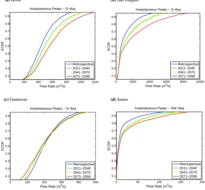
For each lookahead period there are nine projections with 10 simulations each for a total of 90 simulated projections. Each simulated projection is a thirty year time period for a total of 2700 simulated years per lookahead. To evaluate potential changes in flood potential using the 8sq weather generation constraint, the empirical distribution functions by lookahead periods were compared. All 2700 simulated an-nual maximum values were pooled to create a single empiri-cal distribution function for each of three lookahead periods. Figure 5 shows the empirical distribution functions for each of the four basins included in this study for each lookahead period as well as the retrospective period (1951–1997). Each of the four basins has different simulated responses as well as some similarities.

The Boise River Basin shows an increase in annual max-imum flood values with time for essentially all probabili-ties of occurrence. The San Joaquin River Basin has

(a) Boise (b) San Joaquin

0 200 400 600 800 1000 1200

0.1 0.2 0.3 0.4 0.5 0.6 0.7 0.8 0.9

Instantaneous Peaks − S−8sq

Flow Rate (m3/s)

ECDF

Retrospective 2011−2040 2041−2070 2071−2099

0 2000 4000 6000 8000 10000

0.1 0.2 0.3 0.4 0.5 0.6 0.7 0.8 0.9

Instantaneous Peaks − S−8sq

Flow Rate (m3/s)

ECDF

Retrospective 2011−2040 2041−2070 2071−2099

(c) Gunnison (d) James

0 100 200 300 400 500

0.1 0.2 0.3 0.4 0.5 0.6 0.7 0.8 0.9

Instantaneous Peaks − S−8sq

Flow Rate (m3/s)

ECDF

Retrospective 2011−2040 2041−2070 2071−2099

0 50 100 150 200

0.1 0.2 0.3 0.4 0.5 0.6 0.7 0.8 0.9

Instantaneous Peaks − AW−8sq

Flow Rate (m3/s)

ECDF

Retrospective 2011−2040 2041−2070 2071−2099

Fig. 5. Cumulative distributions of annual maximum discharge based on ensemble hydrologic simulation for the periods and basins shown.

Retrospective period is defined as 1951–1997 for all basins. CDFs based on SacSMA simulation of GCM simulated historic climate.

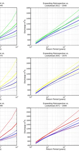
3.3 Expanding retrospective vs. lookahead flood frequency evaluation

As described in Sect. 2.6, the most common method to esti-mate flood risk is to use an expanding retrospective analysis. A second method was also described that only considers the most recent time period to evaluate flood risk. In Sect. 3.2 it was shown that for the four basins there can be varying deviations of simulated future flood potential from those in the retrospective period. The expectation is therefore that the flood frequency estimations will also differ by lookahead period. For example for the Boise River Basin that shows an increase in annual maximum floods for each of the lookahead periods the expanding retrospective approach to evaluate the flood frequency in 2099 will be a blend of all years leading up to 2099 despite the fact that the 2071–2099 period itself does not appear to share much in common with 1951–1997.

(a) Gunnison River above Blue Mesa Dam (b) San Joaquin River above Friant Dam

100 101 102 103

100 200 300 400 500 600 700 800

Return Period (years)

Discharge m

3/s

Expanding Retrospective vs. Lookahead 2011 − 2040

100 101 102 103

0 0.5 1 1.5 2 2.5 3 3.5x 10

4

Return Period (years)

Discharge m

3/s

Expanding Retrospective vs. Lookahead 2011 − 2040

100 101 102 103

100 200 300 400 500 600 700 800 900

Return Period (years)

Discharge m

3 /s

Expanding Retrospective vs. Lookahead 2041 − 2070

100 101 102 103

0 0.5 1 1.5 2 2.5 3 3.5

4x 10

4

Return Period (years)

Discharge m

3/s

Expanding Retrospective vs. Lookahead 2041 − 2070

100 101 102 103

100 200 300 400 500 600 700 800 900

Return Period (years)

Discharge m

3/s

Expanding Retrospective vs. Lookahead 2071 − 2099

100 101 102 103

0 1 2 3 4 5 6x 10

4

Return Period (years)

Discharge m

3/s

Expanding Retrospective vs. Lookahead 2071 − 2099

Fig. 6. Flood Frequency Curves for the locations and lookahead periods as specified. Blue lines represent the Expanding retrospective

(c) James River above Jamestown Dam (d) Boise River above Lucky Peak Dam

100 101 102 103

0 200 400 600 800 1000 1200

Return Period (years)

Discharge m

3/s

Expanding Retrospective vs. Lookahead 2011 − 2040

100 101 102 103

400 600 800 1000 1200 1400 1600 1800

Return Period (years)

Discharge m

3/s

Expanding Retrospective vs. Lookahead 2011 − 2040

100 101 102 103

0 200 400 600 800 1000 1200 1400 1600

Return Period (years)

Discharge m

3/s

Expanding Retrospective vs. Lookahead 2041 − 2070

100 101 102 103

400 600 800 1000 1200 1400 1600 1800

Return Period (years)

Discharge m

3/s

Expanding Retrospective vs. Lookahead 2041 − 2070

100 101 102 103

0 200 400 600 800 1000 1200 1400 1600 1800 2000

Return Period (years)

Discharge m

3/s

Expanding Retrospective vs. Lookahead 2071 − 2099

100 101 102 103

400 600 800 1000 1200 1400 1600 1800 2000 2200

Return Period (years)

Discharge m

3/s

Expanding Retrospective vs. Lookahead 2071 − 2099

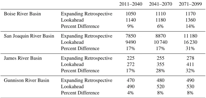
Table 2. 100 year discharge values for each of the basins and lookahead periods as specified as well as percent differences among expanding

retrospective approach and lookahead approach for flood frequency analysis. All values are simulated annual maximum discharges in m3/s rounded to the nearest 10.

2011–2040 2041–2070 2071–2099 Boise River Basin Expanding Retrospective 1050 1110 1170

Lookahead 1140 1180 1360

Percent Difference 9% 6% 14%

San Joaquin River Basin Expanding Retrospective 7850 8870 11 180

Lookahead 9490 10 740 16 230

Percent Difference 17% 17% 31%

James River Basin Expanding Retrospective 225 255 278

Lookahead 272 355 411

Percent Difference 17% 28% 32%

Gunnison River Basin Expanding Retrospective 470 480 490

Lookahead 490 520 530

Percent Difference 4% 8% 8%

For all locations and all lookahead periods the expanding retrospective approach results in a lower estimate of the 100-year flood than the lookahead approach (Table 2). The per-cent differences in the 100-year estimates vary by lookahead period and by basin. For the 2011–2040 lookahead period the smallest percent difference is 4% in the Boise River Basin and the largest percent difference is 17% in the San Joaquin and Jamestown River Basins. For the 2041–2070 lookahead periods the percent differences range from 8% to 28% in the Boise River Basin and the James River Basin, respectively. The smallest percent difference in the 2071–2099 is 8% for the Boise River Basin and the largest percent difference is 32% for the James River Basin. The implication of this re-sult is that to characterize the flood frequency given current methods of fitting log-Pearson III distributions may result in a biased underestimate of the true flood potential. This is an intuitive result given that the empirical distribution functions for each of the locations show an increased trend to bigger floods. The expanding retrospective approach to characteriz-ing the floods continues to give equal weight to floods that occurred during an entirely different climatology.

Perhaps a more important implication is in the context of designing for some lookahead period. Consider if we were to make a flood frequency estimate in 2041 for a structure with a life span until 2099 for each of the four basins an-alyzed in this manuscript. The current methodology would be the expanding retrospective approach over the retrospec-tive period 1951–2041. If the flood potential is increasing through time however at the end of the life span, 2099, of the structure than the flood potential at that time may be very dif-ferent than the 1951–2041. So consider a comparison of the expanding retrospective approach for the 2011–2041 looka-head period as described in Table 2 and the lookalooka-head

ap-proach for 2071–2099. The differences for the four basins are 11%, 52%, 23%, and 45% for the Gunnison, San Joaquin, Boise, and James River Basins, respectively. Therefore, the design would be underestimating the flood with a given risk by between 11% and 52%, depending on the basin, over the life span of the project.

3.4 Uncertainties

The hydrology model used, SAC-SMA, have parameter-ized land surface schemes that are calibrated to past events. It was assumed in this study that these calibrations are reason-able for the future period were kept constant. This approach is first order in that we do not account for developing model physics and parameters. The approach is well supported in the literature of assessing hydrologic impacts through of-fline hydrology models as opposed to hydrology models embedded within climate models (e.g., Miller et al., 2003; Mauer, 2007; Christensen and Lettenmaier, 2007; Purkey et al., 2007). For example, although one of the inputs into the SAC-SMA model is potential evapotranspiration (PET) and PET may be altered in a changing climate, the value was not altered as part of this study. This approach is justified by Miller et al. (2003) that showed that sensitivity to the PET with projected temperature changes was relatively small.

It is also somewhat necessary, to reiterate, the climate models operate at a spatial scale that is inconsistent with the generation of flood flows. We have thus relied upon the cli-mate models for representations of temperature and precipi-tation. We then rely upon a spatial and temporal downscaling techniques to drive the off line hydrology model. Figure 4 shows that the ability of these methods, over the antecedent period, is adequate at reproducing the calibration set floods for non-exceedance probabilities between approximately 0.5 and 0.95.

The results also lead to the need for further research. Each of the four basins responds differently to the climate projec-tions. For a complete understanding of the flood response to climate change it will be important to determine why the responses differ. Key questions are: Is temperature the dom-inant driver, or is precipitation, or some combination? It may also be useful to determine what sorts of generalizations may be derived from these basins to similar basins elsewhere.

4 Conclusions

A set of methods have been developed and presented that allow for the estimation of flood potential given a set of cli-mate projections. These methods are intended to provide an envelope of expected variability of the climate through an equally weighted tercile selection of candidate projections of temperature and precipitation. Through the use of a weather generation scheme and a rainfall runoff tool simulated an-nual maximum discharges are derived for lookahead periods of 2011–2040, 2041–2070, and 2071–2099. These annual maximum discharges are then put into the context of flood frequency analysis. Results indicate that for the four basins analyzed in this study the climate projections result in an in-creased simulated annual maximum flood potential through time. An expanding retrospective approach to characteriz-ing flood hazard may increascharacteriz-ingly underestimate the flood potential as time progresses. Decisions based upon the ex-panding retrospective approach to characterizing flood

fre-quency could be based upon underestimates of future flood potential. Additional work is required to understand the dif-ferences in basin response with the climate forcings, but cur-rent results indicate that more consideration should be given to non-stationarity assumptions when estimating flood risk.

Acknowledgements. This work was funded through the Bureau of

Reclamation Dam Safety Office Technology Development Program as well as the Bureau of Reclamation Research and Development Office. We acknowledge the modeling groups, the Program for Climate Model Diagnosis and Intercomparison (PCMDI) and the WCRP’s Working Group on Coupled Modelling (WGCM) for their roles in making available the WCRP CMIP3 multi-model dataset. Support of this dataset is provided by the Office of Science, US Department of Energy. Review of this manuscript by Blair Greimann, Bureau of Reclamation, Technical Services Center is also greatly appreciated.

Edited by: T. Wagener

References

Alexander, L. V., Zhang, X., Peterson, T. C., Caeser, J., Gleason, B., Klein Tank, A. M. G., Haylock, M., Collins, D., Trewin, B., Rahimzadeh, F., Tagipour, A., Rupa Kumar, K., Revadekar, J., Griffiths, G., Vincent, L., Stephenson, D. B., Burn, J., Aguilar, E., Brunet, M., Taylor, M., New, M., Zhai, P., Rusticucci, M., and Vazquez-Aguirre, J. L.: Global observed changes in daily climate extremes of temperature and precipitation, J. Geophys. Res., 111, D05109, doi:10.1029/2005JD006290, 2006.

Anderson, E. A.: Natinoal Weather Service River Forecast System: Snow Accumulation and Ablation Model, NOAA Tech Memo-randum NWS HYDRO-17, 1973.

Bissel, V. C. and Orwig, C. E.: Calibration of the NWS Model in the Northwest: A Status Report, Proceedings of the 63rd Annual Western Snow Conference, Sparks, NV, 135–138, 1995. Brekke, L. D., Kiang, J. E., Olsen, J. R., Pulwarty, R. S., Raff, D.

A., Turnipseed, D. P., Webb, R. S., and White, K. D.: Climate change and water resources management – A federal perspective, USA Geological Survey Circular 1331, also available at: http: //pubs.usgs.gov/circ/1331/, 65 pp., 2009.

Burnash, R. J., Ferral, R. L., and McQuire, R. A.: A General-ized Streamflow Simulation System, in: Conceptual Modeling for Digital Computers, USA National Weather Service, 1973. Burnash, R. J. C.: The NWS River Forecast System – catchment

modeling, in: Computer Models of Watershed Hydrology, edited by: Singh, V. P., 311–366, 1995.

Cameron, D., Beven, K., and Naden, P.: Flood frequency estima-tion by continuous simulaestima-tion under climate change (with uncer-tainty), Hydrol. Earth Syst. Sci., 4, 393–405, 2000,

http://www.hydrol-earth-syst-sci.net/4/393/2000/.

Christensen, N. S. and Lettenmaier, D. P.: A multimodel ensemble approach to assessment of climate change impacts on the hydrol-ogy and water resources of the Colorado River Basin, Hydrol. Earth Syst. Sci., 11, 1417–1434, 2007,

http://www.hydrol-earth-syst-sci.net/11/1417/2007/.

flood information is available, Water Resour. Res., 33(9), 2089– 2096, 1997.

Cohn, T., Lane, W. M., and Stedinger, J. R.: Confidence Intervals for EMA Flood Quantile Estimates, Water Resour. Res., 37(8), 1695–1706 2001.

Easterling, D. R., Meehl, G. A., Parmesan, C., Changnon, S. A., Karl, T. R., and Mearns, L. O.: Climate Extremes: Observations, Modeling, and Impacts, Science, 2889(5487), 2068–2074, 2000. Emori, S., Hasegawa, A., Suzuki, T., and Dairaku, K.: Validation, parameterization dependence, and future projection of daily pre-cipitation simulated with a high-resolution atmospheric GCM, Geophys. Res. Lett., 32, L06708, doi:10.1029/2004GL022306, 2005.

England Jr., J. F., Salas, J. D., and Jarrett, R. D.: Comparisons of two moments-based estimators that utilize historical and pale-oflood data for the log Pearson type III distribution, Water Re-sour. Res., 39(9), 1243, doi:10.1029/2002WR001791, 2003. Frances, F., Salas, J. D., and Boes, D. C.: Flood frequency

anal-ysis with systematic and historical or paleoflood data based on the two-parameter general extreme value models, Water Resour. Res., 30(6), 1653–1664, 1994.

Gleckler, P. J, Taylor, K. E., and Doutriaux, C.: Performance metrics for climate models, J. Geophys. Res., 113, D06104, doi:10.1029/2007JD008972, 2008.

Griffis, V. W. and Stedinger, J. R.: Incorporating Climate Change and Variability into Bulletin 17B LP3 Model, World Environ-mental and Water Resources Congress 2007: Restoring Our Nat-ural Habitat, American Society of Civil Engineers, 8 pp., 2007. Hamlet, A. F. and Lettenmaier, D. P.: Effects of 20th century

warm-ing and climate variability on flood risk in the western USA, Water Resour. Res., 43, W06427, doi:10.1029/2006WR005099, 2007.

Hirabayashi, Y., Kanae, Shinjiro, K., Emori, S., Oki, T., and Ki-moto, M.: Global projections of changing risks of floods and droughts in a changing climate, Hydrolog. Sci. J., 53(4), 754– 772, 2008.

Interagency Advisory Committee on Water Data (IACWD): Guide-lines for determining flood-flow frequency: Bulletin 17B of the Hydrology Subcommittee, Office of Water Data Coordination, USA Geological Survey, Reston, Va., http://water.usgs.gov/osw/ bulletin17b/bulletin, 183 pp., 1982.

Intergovernmental Panel on Cliamte Change (IPCC): Special Re-port on Emissions Scenarios, edited by: Nakicenovic, N. and Swart, R., Cambridge University Press, Cambridge, UK and New York, NY, USA, 612 pp., 2000.

Intergovernmental Panel on Climate Change (IPCC): Climate Change 2007: The Physical Science Basis. Contribution of Working Group I to the Fourth Assessment Report of the Inter-governmental Panel on Climate Change, edited by: Solomon, S., Qin, D., Manning, M., Chen, Z., Marquis, M., Averyt, K. B., Tignor, M., and Miller, H. L., Cambridge University Press, Cam-bridge, 996 pp., 2007.

Intergovernmental Panel on Climate Change (IPCC): Impacts Adaptation and Vulnerability. Contribution of Working Group II to the Fourth Assessment Report of the Intergovernmental Panel on Climate Change, edited by: Parry, M. L., Canziani, O. F., Palutikof, J. P., van der Linden, P. J., and Hanson, C. E., Cambridge University Press, Cambridge, UK, available at: http://www.ipcc.ch/ipccreports/ar4-wg2.htm, 2007.

Kanae, S., Oki, T., and Kashida, A.: Changes in hourly heavy precipitation at Tokyo from 1890–1999, J. Meteorol. Soc. Jpn., 82(1), 241–247, 2004.

Kunkel, K. E., Easterling, D. R., Redmond, K., and Hubbard, K.: Temporal variations of extreme precipitation events in the United States, J. Geophys. Res., 30, CLM5-1–5-4, 2003.

Lane, W. L. and Cohn T. A.: Expected moments algorithm for flood frequency analysis, in: North American Water and Environment, edited by: Bathala, C. T., Congress 1996, ASCE, Anaheim, Cal-ifornia, 22–28 June 1996.

Manabe, S. and Wetherald, R. T.: On the distribution of climate change resulting from an increase in CO₂content of the atmost-phere, J. Atmos. Sci., 37(1), 99–118, 1980.

Maurer, E. P.: Uncertainty in hydrologic impacts of climate change in the Sierra Nevada, California under two emissions scenarios, Climatic Change, 82, 309–325, 2007.

Maurer, E. P., Brekke, L., Pruitt, T., and Duffy, P. B.: Fine-resolution climate projections enhance regional climate change impact studies, Eos Trans. AGU, 88(47), p. 504, 2007.

Meehl, G. A., Covey, C., Delworth, T., Latif, M., McAvaney, B., Mitchell, J. F. B., Stouffer, R. J., and Taylor, K. E.: The WCRP CMIP3 multi-model dataset: A new era in climate change re-search, B. Am. Meteorol. Soc., 88, 1383–1394, 2007.

Miller, N. L., Bashford, K. E., and Strem, E.: Potential Impacts of Climate Change on California Hydrology, J. Am. Water Resour. As., 39(4), 771–784, 2003.

Milly, P. C. D., Betancourt, J., Falkenmark, M., Hirsch, R. M., Kundzewicz, Z. W., Lettenmaier, D. P., and Stouffer, R. J.: Sta-tionarity is Dead: Whither Water Management?, Science, 319, 573–574, 2008.

O’Connell, D. R. H., Ostenaa, D. A., Levish, D. R., and Klinger, R. E.: Bayesian flood frequency analysis with pa-leohydrologic bound data, Water Resour. Res., 38(5), 1058, doi:10.1029/2000WR000028, 2002.

O’Connell, D. R. H.: Nonparametric Bayesian flood frequency es-timation, J. Hydrol., 313, 79–96, 2005.

Payne, J. R., Wood, A. W., Hamlet, A. F., Palmer, R. N., and Let-tenmaier, D. P.: Mitigatin the effects of climate change on the water resources of the Columbia River Basin, Climatic Change, 62, 233–256, 2004.

Purkey, D. R., Huber-Lee, A., Yates, D. N., Hanemann, M., and Herrod-Jones, S.: Integrating a climate change assessment tool into stakeholder-driven water management decision-making pro-cesses in California, Water Resour. Manag., 21, 315–329, 2007. Reclamation: Appendix R – Sensitivity of Future CVP/SWP

Opera-tions to Potential Climate Change and Associated Sea Level Rise, in CVP/SWP OCAP Biological Assessment, Bureau of Reclama-tion, USA Department of the Interior, 134 pp., 2008.

Salathe, E. P., Mote, P. W., and Wiley, M. W.: Review of scenario selection and downscaling methods for the assessment of climate change impacts on hydrology in the United States Pacific North-west, Int. J. Climatol., 27, 1611–1621, 2007.

Sivapalan, M. and Samuel, J. M.: Transcending lmitations of sta-tionarity and the return period: process-based approach to flood estimation and risk assessment, Hydrol. Process., 23, 1671– 1675, doi:10.1002/hyp.7292, 2009.

hy-drologic information using maximum likelihood techniques, technical report, Cornell Univ., Ithaca, NY, 1988.

Wood, A. W., Maurer, E. P., Kumar, A., and Lettenmaier, D. P.: Long Range Experimental Hydrologic Forecasting for the Eastern U.S., J. Geophys. Res., 107(D20), 4429, doi:10.1029/2001JD000659, 2002.