https://doi.org/10.5194/hess-21-4727-2017 © Author(s) 2017. This work is distributed under the Creative Commons Attribution 3.0 License.
Can spatial statistical river temperature models be transferred
between catchments?
Faye L. Jackson1,2, Robert J. Fryer3, David M. Hannah1, and Iain A. Malcolm2
1School of Geography, Earth and Environmental Science, University of Birmingham, Birmingham, B15 2TT, UK 2Marine Scotland Science, Scottish Government, Freshwater Laboratory, Faskally, Pitlochry, PH16 5LB, UK 3Marine Scotland, Marine Laboratory, 375 Victoria Road, Aberdeen, AB11 9DB, UK
Correspondence to:Faye L. Jackson ([email protected]) Received: 26 January 2017 – Discussion started: 14 February 2017
Revised: 18 August 2017 – Accepted: 21 August 2017 – Published: 21 September 2017
Abstract.There has been increasing use of spatial statistical models to understand and predict river temperature (Tw) from
landscape covariates. However, it is not financially or logis-tically feasible to monitor all rivers and the transferability of such models has not been explored. This paper usesTwdata
from four river catchments collected in August 2015 to assess how well spatial regression models predict the maximum 7-day rolling mean of daily maximum Tw (Twmax)within and between catchments. Models were fitted for each catchment separately using (1) landscape covariates only (LS models) and (2) landscape covariates and an air temperature (Ta) met-ric (LS_Ta models). All the LS models included upstream catchment area and three included a river network smoother (RNS) that accounted for unexplained spatial structure. The LS models transferred reasonably to other catchments, at least when predicting relative levels ofTwmax. However, the predictions were biased when mean Twmax differed between catchments. The RNS was needed to characterise and predict finer-scale spatially correlated variation. Because the RNS was unique to each catchment and thus non-transferable, pre-dictions were better within catchments than between catch-ments. A single model fitted to all catchments found no in-teractions between the landscape covariates and catchment, suggesting that the landscape relationships were transferable. The LS_Ta models transferred less well, with particularly poor performance when the relationship with the Ta metric was physically implausible or required extrapolation outside the range of the data. A single model fitted to all catchments found catchment-specific relationships between Twmax and theTametric, indicating that theTa metric was not
transfer-able. These findings improve our understanding of the
trans-ferability of spatial statistical river temperature models and provide a foundation for developing new approaches for pre-dictingTw at unmonitored locations across multiple
catch-ments and larger spatial scales.
Copyright statement. The works published in this journal are distributed under the Creative Commons Attribution 3.0 License. This license does not affect the Crown copyright work, which is re-usable under the Open Government Licence (OGL). The Creative Commons Attribution 3.0 License and the OGL are interoperable and do not conflict with, reduce or limit each other.
© Crown copyright 2017
1 Introduction
management. Large-scale models are required to provide in-formation at the spatial scales appropriate to management de-cisions, i.e. catchment (Chang and Psaris, 2013; Hrachowitz et al., 2010; Imholt et al., 2011, 2013; Jackson et al., 2017b; Steel et al., 2016), regional (Hill et al., 2013; Isaak et al., 2012; Ruesch et al., 2012) and national scales.
Although process-based models provide important mech-anistic understanding at small spatial scales, their intensive data requirements prohibit their use at larger scales (Jack-son et al., 2016). In contrast, empirical models of Tw rely
onTwobservations and explanatory covariates (e.g. altitude
or air temperature) which can often be derived remotely at relatively low cost. The development of affordable, reliable, accurate Tw data loggers has led to a rapid increase in Tw
monitoring (Sowder and Steel, 2012), to the point that staff time, data storage and quality control are often now the great-est limitations on data collection (Jackson et al., 2016). At the same time, there have been substantial developments in spa-tial statistical modelling approaches (Ver Hoef et al., 2006, 2014; Ver Hoef and Peterson, 2010; Isaak et al., 2014; Jack-son et al., 2017b; O’Donnell et al., 2014; PeterJack-son et al., 2013; Rushworth et al., 2015), monitoring network design (Dobbie et al., 2008; Jackson et al., 2016; Som et al., 2014), spatial datasets (e.g. shapefiles incorporating covariates such as in “The National Stream Internet Project” (Isaak et al., 2011) or gridded air temperature datasets (Perry and Hollis, 2005a, b)) and spatial analysis tools (Isaak et al., 2011, 2014; Peterson et al., 2013; Peterson and Ver Hoef, 2014).
While continuous river temperature data are routinely col-lected in some areas, resulting in large regional tempera-ture datasets and associated models (e.g. Wehrly et al., 2009; Moore et al., 2013), this is far from universal. In many cases, financial and logistical considerations limit data collection, making it impractical to monitor all rivers. For example, in Scotland, there are 16 006 river catchments (unique rivers running to the sea), including 629 catchments >10 km2, but there was no systematic nationwide quality-controlled river temperature data collection until 2015 (Jackson et al., 2016). For management purposes, it is therefore often nec-essary to predict Tw at unmonitored locations, both within
(Hrachowitz et al., 2010; Jackson et al., 2017b; Peterson and Urquhart, 2006) and between catchments (Isaak et al., 2014). In recent years, it has become increasingly common to de-velop and apply spatial statistical river network models that incorporate network covariance structure to predict spatial variability in river temperature (e.g. Isaak et al., 2014; Jack-son et al., 2017b). It is widely acknowledged that these mod-els can dramatically improve predictions of river temperature where sufficient observational data exist, but the covariance component of the predictions cannot typically be transferred between catchments. Despite these important issues, there has not yet been an assessment of the transferability of spa-tial statisticalTwmodels between catchments; i.e. the ability
of a model developed in one catchment to predictTw in
an-other. This paper investigates the ability of spatial statistical
Twmodels to predictTwat unmonitored locations within and between catchments.
The principles explored in this paper are likely to be rel-evant to other water temperature metrics so, for brevity, this study focuses on maximum summer temperature, a metric which is prevalent in the recent literature, reflecting its im-portance for the survival of cold-water-adapted fish (Chang and Psaris, 2013; Hrachowitz et al., 2010; Jackson et al., 2017b; Malcolm et al., 2008; Marine and Cech, 2004).
Models are fitted using two sets of covariates. The first set contains landscape covariates which can be generated from readily available spatial datasets and have been the focus of many previous studies of spatial variability in river tempera-ture (e.g. Hrachowitz et al., 2010). Due to increasing interest in the use of air temperature (Ta) to predict spatial variability in water temperature (e.g. Jonkers and Sharkey, 2016), the second set contains a metric of air temperature in addition to landscape covariates.
The paper addresses the objectives to
1. develop statistical models for predicting maximum summer water temperature from landscape covariates in four separate river catchments,
2. determine whether models containing an air tempera-ture metric explain more of the variation in maximum summer water temperature than those only containing landscape covariates,
3. assess the transferability of models containing only landscape covariates or both landscape and air tempera-ture covariates between catchments and
4. produce single models of maximum summer water tem-perature for all four catchments using both sets of co-variates and consider their potential for transferability at larger (e.g. national) scales.
2 Methodology
2.1 Water temperature data and metric
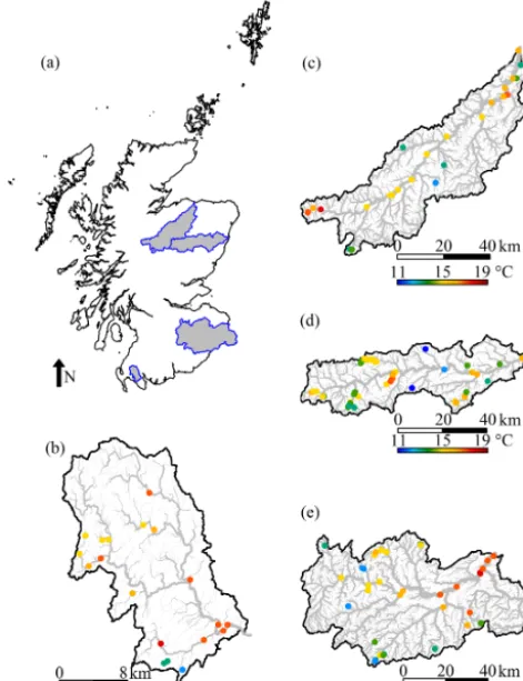
Tw data were obtained from monitoring sites in four catch-ments: the Bladnoch in western Scotland, and the Dee (Ab-erdeenshire), Spey and Tweed in eastern Scotland (Fig. 1). These catchments are Special Areas of Conservation for At-lantic salmon and form part of the Scotland River Temper-ature Monitoring Network (SRTMN) (Jackson et al., 2016). Details of the network, including design and quality-control procedures, are given in Jackson et al. (2016). The catch-ments all contain an adequate number ofTw data loggers to
developTwmodels on a single-catchment basis, with 59, 34,
Figure 1.Study catchments and spatial patterns ofTwmax for
Au-gust 2015 (Jackson et al., 2017a).(a)Catchment positions in Scot-land,(b)the River Bladnoch catchment,(c)River Spey catchment, (d)River Dee catchment and(e)River Tweed catchment. Some fea-tures of this map are based on digital spatial data licensed from the Centre for Ecology & Hydrology, © NERC (CEH) and con-tains Ordnance Survey data © Crown copyright and database right (2016). Catchment boundaries are from SEPA (2009).
Data were collected at 15 min intervals throughout Au-gust 2015. The maximum temperature was calculated for each day and used to produce a 7-day rolling mean of max-imum temperatures. The metric of maxmax-imum temperatures used in this study (Twmax) was the maximum value of this 7-day rolling mean (Jackson et al., 2017a). This metric was preferred to a single observation ofTw, as it characterises the occurrence of sustained high temperatures which are thought to be most ecologically damaging.
2.2 Model covariates
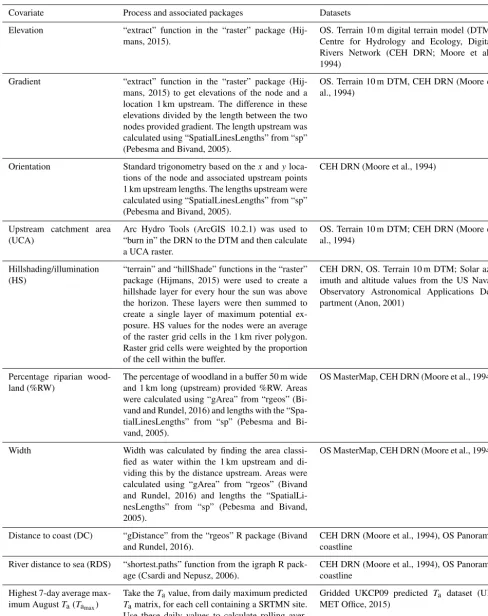
Detailed discussion of the landscape covariates and their cal-culation can be found in Jackson et al. (2016). In brief, the covariates were elevation (Elevation), upstream catchment area (UCA), percentage riparian woodland (%RW), hillshad-ing/channel illumination (HS), channel width (Width), chan-nel gradient (Gradient), chanchan-nel orientation (Orientation),
distance to coast (DC) and distance to the sea along the river (RDS). Table 1 summarises how the covariates were calcu-lated. Before model fitting, gradient, UCA and width were log transformed to reduce skewness, and HS was centred by subtracting the median value from all observations.
An air temperature metric (Tamax)was calculated for each site from the gridded UKCP09Tadataset (available from the
UK MET Office); see Perry and Hollis (2005a, b) for details of this dataset. Analogous to the calculation ofTwmax,Tamax was given by the maximum of the 7-day rolling mean of daily maximum air temperatures in August 2015.
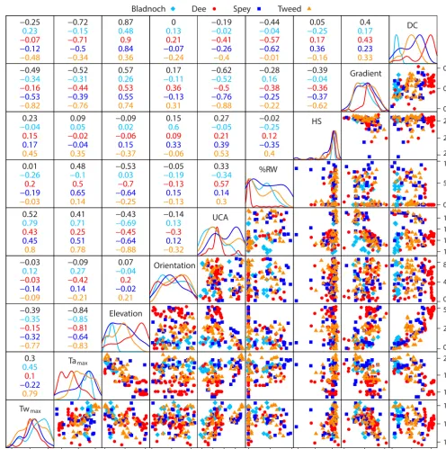
Figure 2 illustrates the distribution and correlation among covariates included in the single- or multi-catchment mod-els (excluding strongly correlated (>0.8) covariate pairs; see below for details) for each of the four catchments and for the global (four-catchment) dataset.
2.3 Modelling
A total of ten models ofTwmax were developed: two models for each of the four river catchments using either (1) land-scape covariates only (LS models) or (2) landland-scape covari-ates andTamax (LS_Tamodels) and two models for all four catchments combined, again using either (1) landscape co-variates only (multi-catchment LS model) or (2) landscape covariates and Tamax (multi-catchment LS_Ta model). The modelling process differs slightly between the single and multi-catchment models and these are described in turn. All analysis was done in R version 3.2.3 (R Core Team, 2015). 2.3.1 Single-catchment models
The set of covariates was first reduced to avoid problems of collinearity. If two covariates were strongly correlated (Pearson correlation coefficient of more than 0.8) in any one catchment, one of the covariates was dropped from the set available for modelling for all catchments. This ensured all the LS models were based on a common set of covariates (UCA, %RW, HS, Orientation, DC) as were the LS_Ta
mod-els (Tamax, UCA, %RW, HS, Orientation, DC).
The relationship between Twmax and the covariates was explored using generalised additive models (GAMs) with Gaussian errors and an identity link (Wood, 2001). A “full” model was first fitted, which included all the available covari-ates from the reduced dataset and a river network smoother (RNS) (see below). The model can be conveniently written in R formula syntax as
Twmax∼s(covariate1)+. . .+s(covariaten)+RNS, (1) wherenis the number of covariates (n=5, 6 for LS, LS_Ta
models, respectively),s(covariatei)denotes that covariate i
sim-Table 1.Covariate calculations. All calculations were in R version 3.2.3 (R Core Team, 2015) except where specified.
Covariate Process and associated packages Datasets
Elevation “extract” function in the “raster” package (Hij-mans, 2015).
OS. Terrain 10 m digital terrain model (DTM) Centre for Hydrology and Ecology, Digital Rivers Network (CEH DRN; Moore et al., 1994)
Gradient “extract” function in the “raster” package (Hij-mans, 2015) to get elevations of the node and a location 1 km upstream. The difference in these elevations divided by the length between the two nodes provided gradient. The length upstream was calculated using “SpatialLinesLengths” from “sp” (Pebesma and Bivand, 2005).
OS. Terrain 10 m DTM, CEH DRN (Moore et al., 1994)
Orientation Standard trigonometry based on thexandy loca-tions of the node and associated upstream points 1 km upstream lengths. The lengths upstream were calculated using “SpatialLinesLengths” from “sp” (Pebesma and Bivand, 2005).
CEH DRN (Moore et al., 1994)
Upstream catchment area (UCA)
Arc Hydro Tools (ArcGIS 10.2.1) was used to “burn in” the DRN to the DTM and then calculate a UCA raster.
OS. Terrain 10 m DTM; CEH DRN (Moore et al., 1994)
Hillshading/illumination (HS)
“terrain” and “hillShade” functions in the “raster” package (Hijmans, 2015) were used to create a hillshade layer for every hour the sun was above the horizon. These layers were then summed to create a single layer of maximum potential ex-posure. HS values for the nodes were an average of the raster grid cells in the 1 km river polygon. Raster grid cells were weighted by the proportion of the cell within the buffer.
CEH DRN, OS. Terrain 10 m DTM; Solar az-imuth and altitude values from the US Naval Observatory Astronomical Applications De-partment (Anon, 2001)
Percentage riparian wood-land (%RW)
The percentage of woodland in a buffer 50 m wide and 1 km long (upstream) provided %RW. Areas were calculated using “gArea” from “rgeos” (Bi-vand and Rundel, 2016) and lengths with the “Spa-tialLinesLengths” from “sp” (Pebesma and Bi-vand, 2005).
OS MasterMap, CEH DRN (Moore et al., 1994)
Width Width was calculated by finding the area classi-fied as water within the 1 km upstream and di-viding this by the distance upstream. Areas were calculated using “gArea” from “rgeos” (Bivand and Rundel, 2016) and lengths the “SpatialLi-nesLengths” from “sp” (Pebesma and Bivand, 2005).
OS MasterMap, CEH DRN (Moore et al., 1994)
Distance to coast (DC) “gDistance” from the “rgeos” R package (Bivand and Rundel, 2016).
CEH DRN (Moore et al., 1994), OS Panorama coastline
River distance to sea (RDS) “shortest.paths” function from the igraph R pack-age (Csardi and Nepusz, 2006).
CEH DRN (Moore et al., 1994), OS Panorama coastline
Highest 7-day average max-imum AugustTa(Tamax)
Take theTavalue, from daily maximum predicted Tamatrix, for each cell containing a SRTMN site. Use these daily values to calculate rolling aver-ages, then select the highest for each site.
[image:4.612.55.543.93.709.2]Figure 2.Distributions and inter-relationships betweenTwmaxand covariates. Scatter plots of the relationships are shown below the diagonal,
kernel density plots of the individual covariates in the diagonal (scaled to have the same maximum value) and correlation coefficients above the diagonal. Numbers in black indicate the correlation coefficients where data are pooled across all catchments.
plicity of Twmax responses to the covariates. The RNS is in-cluded to account for spatial structure in the data that can-not be explained by the covariates. The RNS is a modified version of that developed by O’Donnell et al. (2014), with the amount of smoothness at a confluence controlled by the proportional influence of upstream tributaries weighted by Strahler river order (Strahler, 1957) and fitted using a set of
Spey and Dee RNSs due to correlations with DC. In the LS_Tamodels, base 2 was also removed from the Spey RNS due to correlation withTamax. The model was fitted by max-imum likelihood using the “mgcv” package (Wood, 2016) in R.
All possible subsets of the full model were then fitted. The final model was that with the lowest Bayesian information criterion (BIC) or Akaike information criterion corrected for small sample size (AICc) that contained no terms signifi-cant at the 5 % level. The choice of information criterion was based on the desire to penalise more complex models that would be unlikely to transfer well (Millidine et al., 2016). Thus, BIC was used for the Dee and Tweed where there were more sites, and AICc was used for the Bladnoch and Spey where there were fewer sites. Terms in the final model with 1 df were replaced by linear terms.
In common with similar modelling studies (Hrachowitz et al., 2010; Imholt et al., 2011; Jackson et al., 2017b; Ruesch et al., 2012), no interactions were considered between covari-ates due to data constraints.
2.3.2 Multi-catchment models
Covariates were excluded if they were strongly correlated (>
0.8) across the entire multi-catchment dataset. The reduced set of covariates was elevation, UCA, %RW, HS, gradient and orientation for the LS model, and Tamax, UCA, %RW, HS, gradient and orientation for the LS_Tamodel. The RNS
basis functions were the same as those included in the single-catchment models.
A “starting” model was fitted of the following form:
Twmax∼Catchment+s(covariate1)+. . .
+s(covariaten)+RNS : Catchment,
where Catchment is a categorical variable allowing a dif-ferent mean level for each catchment and RNS : Catchment denotes a separate RNS for each catchment. The covariate smoothers were given a maximum of 2 df and the RNS a maximum of 7 df for each catchment. The model was then re-fined in a backwards and forwards stepwise procedure which considered (a) replacing smooth covariate effects by linear terms and then dropping them altogether; (b) dropping the RNS by Catchment term altogether; and (c) adding interac-tions between the covariates (either linear or smoothed) and Catchment. An interaction between a covariate and Catch-ment would indicate inter-catchCatch-ment differences in the rela-tionship betweenTwmaxand the covariate, suggesting that the model might not transfer well to new catchments. Interac-tions between the covariates were not considered. Model se-lection was based on BIC. Finally, any non-significant terms
(p >0.05) in the final model were removed.
2.3.3 Model performance and transferability of single-catchment models
The ability of single-catchment models to predict Twmax within the catchment they were developed (the donor catch-ment) was assessed using leave-one-out cross validation. Each site was removed in turn, the final model was refit-ted, and thenTwmax was predicted at the missing site using (a) using all model terms (i.e. the covariates and the RNS if present) and (b) only covariates (i.e. excluding the columns in the model matrix relating to the RNS). The prediction us-ing all model terms should outperform that usus-ing only covari-ates because it incorporcovari-ates the extra information about spa-tial structure that is captured by the RNS. However, a RNS from one catchment cannot be used to predict in another be-cause the river networks will differ. The prediction using only covariates therefore provides a benchmark for assessing the transferability of models between catchments, since it mea-sures how well a model will transfer to a catchment that is identical in all but its river network.
Transferability to another catchment (the target ment) was assessed by using the model from the donor catch-ment to predict Twmax at the monitoring sites in the target catchment. As RNSs cannot be transferred, only covariates were used in the predictions (i.e. the columns in the model matrix due to the RNS were ignored).
Three performance metrics were calculated: root mean square error (RMSE) (Eq. 1), which measures overall per-formance (accuracy), standard deviation (SD) (Eq. 2), which measures how well a model can predict within-catchment spatial variability (precision), and bias (Eq. 3).
RMSE=
v u u t 1
n
n
X
s=1
(xˆs−xs)2 (2)
SD=
v u u t 1
n
n
X
s=1
((xˆs− ¯ˆx)−(xs− ¯x))2 (3)
bias= ¯ˆx− ¯x, (4)
where xs and xˆs are the observed and predicted Twmax at sites, x¯ andx¯ˆ are the mean observed and predictedTwmax
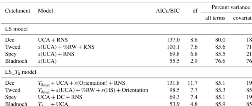
Table 2.LS model and LS_Tamodel for each catchment, with the percent variance explained by the model (all terms) and the same model but with the RNS omitted (covariates).
Catchment Model AICc/BIC df Percent variance
all terms covariates
LS model
Dee UCA+RNS 137.0 8.8 80.0 18.3
Tweed s(UCA)+%RW+RNS 100.1 7.6 85.6 71.7
Spey s(UCA)+RNS 69.8 6.8 85.5 21.8
Bladnoch s(UCA) 55.5 2.9 76.6 76.6
LS_Tamodel
Dee Tamax+UCA+s(Orientation)+RNS 131.8 11.7 85.1 19.9
Tweed Tamax+s(UCA)+%RW+s(HS)+Orientation 98.5 7.7 85.3 85.3
Spey UCA+DC+RNS 69.3 7.4 85.1 19.9
Bladnoch Tamax+UCA 53.9 4.8 85.9 85.9
3 Results
Across Scotland, August 2015 was wetter than the 1981– 2010 mean (MET Office, 2016) and this was reflected in relatively low Tw. Rainfall in eastern Scotland (which
cov-ers the Spey, Dee and Tweed) was 107 % of the 1981–2010 mean, whereas rainfall in western Scotland (which covers the Bladnoch) was only 98 % of the 1981–2010 mean (MET Of-fice, 2016). Maximum air temperature was the same in east-ern Scotland as the 1981–2010 mean maximum and 0.2◦C cooler in western Scotland over the same period (MET Of-fice, 2016).
Figure 1 shows the spatial variability in Twmax across the four catchments and Fig. 2 summarises the distribution of Twmax by catchment (bottom left diagonal panel). Me-dianTwmax in the Dee (15.1
◦C), Tweed (15.6◦C) and Spey (15.6◦C) was broadly similar, but medianTw
maxin the Blad-noch (16.4◦C) was approximately 1◦C higher (Fig. 2). The range ofTwmax was 5.7, 5.9, 6.0 and 5.5
◦C in the Bladnoch, Dee, Spey and Tweed, respectively (Fig. 2).
3.1 Single-catchment models
All four LS models were simple (Table 2), explained much of the variance inTwmax (76.6–85.6 %) and contained similar positive relationships betweenTwmax and UCA (Fig. 3). This relationship was near linear until approximately 100 km2and then levelled off in the Bladnoch (Fig. 3d), and it was smooth, but near linear in the Spey and the Tweed (Fig. 3b, c) and linear in the Dee (Fig. 3a). The magnitude of the effect was similar across catchments at approximately 4◦C. Three mod-els contained a RNS, which explained much of the variance: 61.7, 13.9 and 63.7 % in the Dee, Tweed and Spey, respec-tively (Table 2). The Tweed model also had a negative linear effect of %RW.
The LS_Tamodels always had a better BIC/AICc than the
corresponding LS models but were typically more complex, always required more df and only explained a greater percent of the variance in the Bladnoch and the Tweed (Table 2). For the Tweed, the LS_Ta model used only covariates, whereas
the LS model required a RNS to account for unexplained spa-tial structure. For the Bladnoch, the LS_Ta model included
UCA andTamax, whereas the LS model only included UCA. In common with the LS models, UCA was in all the LS_Ta
models (Table 2) and the direction, shape and magnitude of the effects were consistent with the LS models (Fig. 4, top row).Tamaxwas in all the LS_Tamodels except the Spey (Ta-ble 2). There was a positive linear relationship betweenTwmax
andTamax in the Dee and Tweed (Fig. 4e, f) and a U-shaped response in the Bladnoch which is physically implausible, increasingly so when extended beyond the range ofTamax ob-served in the Bladnoch (Fig. 4g). Orientation had a small pos-itive effect onTwmax in both the Dee and Tweed (Fig. 4h, i) with higher temperatures for a north–south orientation than an east–west orientation. There was also a negative linear ef-fect of %RW and a positive smoothed efef-fect of HS in the Tweed and a positive linear effect of DC in the Spey (Fig. 4j, k, l, respectively).
3.2 Transferability of single-catchment models
The transferability of the LS and LS_Ta models is sum-marised by their RMSE, bias and standard deviation in Ta-ble 3 and illustrated in Figs. 5 and 6, respectively. All the models performed well within catchments (i.e. in the catch-ments where they were developed) when all model terms (i.e. both covariates and the RNS) were used in the predic-tions, with a bias of<0.1◦C in absolute value and a RMSE of<1◦C. The LS_Tamodels always had a lower RMSE than
(exclud-Figure 3.LS model effects with pointwise 95 % confidence bands:(a)Dee UCA,(b)Tweed UCA,(c)Spey UCA,(d)Bladnoch UCA and (e)Tweed %RW.
ing RNS), with a median RMSE of 1.2◦C and a maximum RMSE of 1.8◦C.
The rest of this section focuses on the predictions, both within and between catchments, using only the covariates. For the catchments in eastern Scotland (Dee, Tweed and Spey), the RMSE, bias and standard deviation of any model were broadly similar whether they were used to predict for the donor catchment or for the other two target catchments. The RMSE of the LS models tended to be lower than that
of the LS_Tamodels (median 1.3 and 1.7◦C, respectively).
The LS and LS_Tamodels both had median absolute biases of 0.3◦C and median standard deviations of 1.1 and 1.4◦C, respectively. RMSE is a combination of bias and standard de-viation, so the RMSE of both sets of models was generally dominated by the standard deviation.
[image:8.612.128.469.65.547.2]Figure 4.LS_Tamodel effects with pointwise 95 % confidence bands. Each column corresponds to a catchment and each row to a covariate. (a)Dee UCA,(b)Tweed UCA,(c)Spey UCA,(d)Bladnoch UCA,(e)DeeTamax,(f)TweedTamax,(g)BladnochTamax,(h)Dee Orientation,
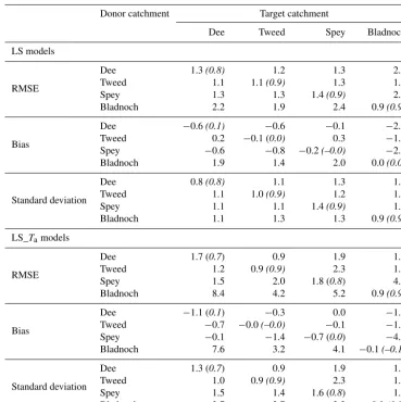
Table 3.Transferability of LS and LS_Tamodels. The values in normal font are for predictions using only covariates (any RNS information is ignored). The values in italics are for predictions when the target and donor catchments are the same and all model terms are used (both covariates and the RNS).
Donor catchment Target catchment
Dee Tweed Spey Bladnoch
LS models
RMSE
Dee 1.3(0.8) 1.2 1.3 2.3
Tweed 1.1 1.1(0.9) 1.3 1.9
Spey 1.3 1.3 1.4(0.9) 2.5
Bladnoch 2.2 1.9 2.4 0.9(0.9)
Bias
Dee −0.6(0.1) −0.6 −0.1 −2.0
Tweed 0.2 −0.1 (0.0) 0.3 −1.7
Spey −0.6 −0.8 −0.2(–0.0) −2.3
Bladnoch 1.9 1.4 2.0 0.0(0.0)
Standard deviation
Dee 0.8(0.8) 1.1 1.3 1.2
Tweed 1.1 1.0(0.9) 1.2 1.0
Spey 1.1 1.1 1.4(0.9) 1.0
Bladnoch 1.1 1.3 1.3 0.9(0.9)
LS_Tamodels
RMSE
Dee 1.7 (0.7) 0.9 1.9 1.9
Tweed 1.2 0.9(0.9) 2.3 1.5
Spey 1.5 2.0 1.8 (0.8) 4.2
Bladnoch 8.4 4.2 5.2 0.9(0.9)
Bias
Dee −1.1 (0.1) −0.3 0.0 −1.4
Tweed −0.7 −0.0(–0.0) −0.1 −1.0
Spey −0.1 −1.4 −0.7 (0.0) −4.1
Bladnoch 7.6 3.2 4.1 −0.1(–0.1)
Standard deviation
Dee 1.3 (0.7) 0.9 1.9 1.2
Tweed 1.0 0.9(0.9) 2.3 1.1
Spey 1.5 1.4 1.6 (0.8) 1.1
Bladnoch 3.7 2.7 3.3 0.9(0.9)
(Fig. 2). The Bladnoch models always overpredictedTwmaxin the other catchments and the Dee, Tweed and Spey models all underpredicted Twmax in the Bladnoch (Figs. 5, 6). This often led to substantial bias and hence RMSE. The Bladnoch LS_Ta model had the largest biases, which were also due to
the implausible relationship with Tamax (Fig. 4g). The Dee, Tweed and Spey had reasonable standard deviations when transferred to the Bladnoch (median 1.0 and 1.1◦C for the LS and LS_Tamodels, respectively) which suggests that, despite having poor RMSE, the models still could be used to predict areas of relatively high or low Twmax within the Bladnoch (rather than absolute values of Twmax). The same is true of the Bladnoch LS models when transferred to the Dee, Tweed and Spey (median standard deviation 1.3◦C). However, the Bladnoch LS_Tamodel had a high standard deviation
(me-dian 3.3◦C) when transferred to the Dee, Tweed and Spey, again due to the implausible relationship withTamax.
3.3 Multi-catchment models
10 12 14 16 18 20
10
12
14
16
18
20
Dee observed Tw
Predicted T
w
(a)
10 12 14 16 18 20
10
12
14
16
18
20
Tweed observed Tw
Predicted T
w
(b)
10 12 14 16 18 20
10
12
14
16
18
20
Spey observed Tw
Predicted T
w
(c)
10 12 14 16 18 20
10
12
14
16
18
20
Bladnoch observed Tw
Predicted T
w
(d)
Dee model in range Dee model out range Dee model with RNS
Tweed model in range Tweed model out range Tweed model with RNS
Spey model in range Spey model out range Spey model with RNS
[image:11.612.101.492.67.466.2]Bladnoch model in range Bladnoch model out range Bladnoch model with RNS
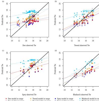
Figure 5.LS model transferability. Panels(a),(b),(c)and(d)show predictedTwmaxwhen the target catchment is the Dee, Tweed, Spey and
Bladnoch, respectively. The colours and symbols indicate the donor catchment: Dee (red circles), Tweed (orange triangles), Spey (dark blue squares) and Bladnoch (light blue diamonds). Filled (open) symbols indicate sites in (out) of the environmental range of the donor catchment. When the target and donor catchments are the same, the coloured points are based on predictions using only covariates; the grey symbols show the corresponding predictions based on the covariates and the RNS. The dashed lines are robust regression lines of observed against predicted values. Models which transfer well have points falling close to the 1:1 line.
Table 4.Multi-catchment LS and LS_Tamodels, with the percent variance explained by the model (all terms) and when the RNS is omitted (covariates).
Model BIC df Percent variance
all terms covariates
Multi-catchment LS model
Catchment+s(UCA)+%RW+Elevation+RNS : Catchment 379.3 24.8 84.4 51.9
Multi-catchment LS_Tamodel
[image:11.612.86.512.591.693.2]10 12 14 16 18 20
10
15
20
25
30
Dee observed Tw
Predicted T
w
(a)
10 12 14 16 18 20
10
15
20
25
30
Tweed observed Tw
Predicted T
w
(b)
10 12 14 16 18 20
10
15
20
25
30
Spey observed Tw
Predicted T
w
(c)
10 12 14 16 18 20
10
12
14
16
18
20
Bladnoch observed Tw
Predicted T
w
(d)
Dee model in range Dee model out range Dee model with RNS
Tweed model in range Tweed model out range Tweed model with RNS
Spey model in range Spey model out range Spey model with RNS
[image:12.612.102.491.71.472.2]Bladnoch model in range Bladnoch model out range Bladnoch model with RNS
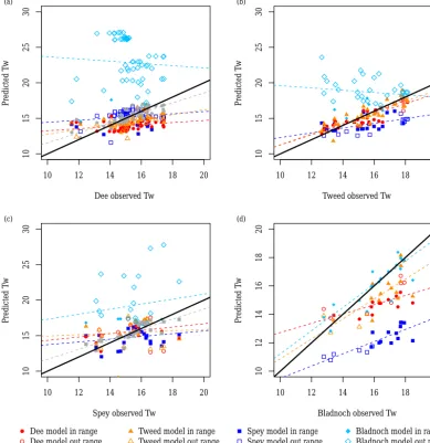
Figure 6.LS_Tamodel transferability. Panels(a),(b),(c)and(d)show predictedTwmaxwhen the target catchment is the Dee, Tweed, Spey
and Bladnoch, respectively. The colours and symbols indicate the donor catchment: Dee (red circles), Tweed (orange triangles), Spey (dark blue squares) and Bladnoch (light blue diamonds). Filled (open) symbols indicate sites in (out) of the environmental range of the donor catchment. When the target and donor catchments are the same, the coloured points are based on predictions using only covariates; the grey symbols show the corresponding predictions based on the covariates and the RNS. The dashed lines are robust regression lines of observed against predicted values. Models which transfer well have points falling close to the 1:1 line.
explain less of the variance than in the single-catchment models (Tables 3, 4).
The multi-catchment LS_Ta model explained 83.2 % of
the variance and contained Catchment, UCA, %RW, Tamax and a RNS for each catchment (Table 4, Fig. 8). None of the landscape covariates interacted with catchment. However, the Tamax relationship did interact with catchment (Fig. 8a– d), with positive relationships in the Dee and Tweed, and negative (albeit non-significant) relationships in the Spey and Bladnoch. This suggests that relationships withTamax are non-transferable andTamax would not be a good predictor of
Twmaxin new catchments.
4 Discussion
−4
−2
0
1
2
UCA (km2)
P
artial ef
fect
C
1 10 100 1000
(a)
0 20 40 60 80 100
−4
−2
0
1
2
%RW
P
artial ef
fect
C
(b)
0 100 200 300 400 500
−4
−2
0
1
2
Elevation (m)
P
artial ef
fect
C
(c)
−4
−2
0
1
2
Catchment
P
artial ef
fect
C
Tweed Dee Bladnoch Spey
[image:13.612.97.496.68.334.2](d)
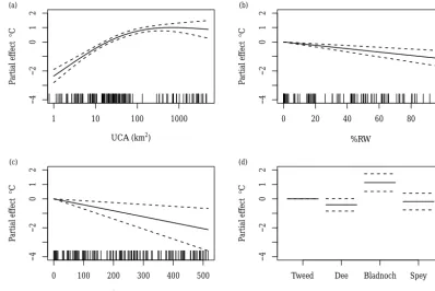
Figure 7.Multi-catchment LS model effects with pointwise 95 % confidence bands:(a)UCA,(b)%RW,(c)Elevation and(d)Catchment.
transferred these models between catchments. Models con-taining only landscape covariates typically contained simi-lar covariates and covariate responses, and performed bet-ter than models containingTamax when transferred between catchments. A physically implausible model transferred par-ticularly poorly. The covariates alone often explained much less of the spatial temperature variability than when a RNS was added but provided the only means of predicting temper-ature in new catchments with no or limited data (a minimum of 19 loggers was required to fit the full models including covariates and RNS). A single model fitted to all four catch-ments suggested common responses to landscape covariates but inter-catchment differences in mean temperature and in the relationships betweenTwmaxandTamax. These findings are discussed in more detail below.
4.1 Twmaxresponses to landscape covariates
The single-catchment LS models contained similar covari-ates with comparable effect sizes and response shapes which suggested that transferability between catchments could be reasonably successful. This was confirmed by the lack of sig-nificant interactions with Catchment in the multi-catchment model. However, when there are inter-catchment differences in mean temperature, the models might only be good pre-dictors of relative values of Twmax within a new catchment (i.e. areas of higher or lowerTwmax)rather than absolute val-ues. It is also unclear how well the models would perform in years with differing hydroclimatic characteristics. This study
was conducted in a single year with relatively low tempera-tures and high flows. In a hotter, drier year it might be ex-pected that between-site differences would be greater. Under such circumstances, the current models may not provide ac-curate predictions of absolute temperatures or inter-site dif-ferences without refitting.
All of theTwmax responses to landscape covariates (across all models) were physically plausible and hence broadly transferable (Smith et al., 2016). UCA (which was in all the models) is a proxy for discharge, water volume and thermal capacity (Chang and Psaris, 2013; Hannah et al., 2008). Higher UCAs are generally associated with larger wa-ter volumes which have a greawa-ter thermal capacity, taking longer to warm but also retaining heat for longer (Chang and Psaris, 2013; Imholt et al., 2011). Elevation reflects adiabatic lapse rates which reduce temperatures with increasing alti-tude (Hrachowitz et al., 2010; Jackson et al., 2017b). The negative relationship betweenTwmaxand %RW woodland oc-curs because riparian shading reduces the amount of incident shortwave radiation reaching the river during daylight hours (Garner et al., 2014; Hannah et al., 2008; Moore et al., 2005). The positive relationship betweenTw and HS is consistent
with greaterTw in locations with lower shading effects and
greater direct shortwave contributions (illumination).Twwas
differ-14 16 18 20 22
−4
−2
0
2
4
Dee Tamax effect C
P
artial ef
fect
C
(a)
14 16 18 20 22
−4
−2
0
2
4
Tweed Tamax effect C
P
artial ef
fect
C
(b)
14 16 18 20 22
−4
−2
0
2
4
Spey Tamax effect C
P
artial ef
fect
C
(c)
14 16 18 20 22
−4
−2
0
2
4
Bladnoch Tamax effect C
P
artial ef
fect
C
(d)
−4
−2
0
2
4
UCA (km2)
P
artial ef
fect
C
1 10 100 1000
(e)
0 20 40 60 80 100
−4
−2
0
2
4
%RW
P
artial ef
fect
C
(f)
−4
−2
0
2
4
Catchment
P
artial ef
fect
C
Tweed Dee Bladnoch Spey
[image:14.612.112.483.65.565.2](g)
Figure 8.Multi-catchment LS_Tamodel effects with pointwise 95 % confidence bands:(a)DeeTamax,(b)TweedTamax,(c)SpeyTamax,
(d)BladnochTamax,(e)UCA,(f)%RW and(g)Catchment.
ing specific heat capacities of land and sea, specifically ther-mal buffering of relatively cooler sea during summer months (Chang and Psaris, 2013; Hrachowitz et al., 2010).
4.2 Tw–Tarelationships
In contrast to the LS models, one LS_Ta model included
a physically implausible relationship that would not be
where the relationships betweenTwmax andTamax were plau-sible, they were inconsistent between catchments in terms of effect size and direction, as indicated by the varying re-sponses in the single-catchment models and the interaction with Catchment in the multi-catchment model. For example, in the latter, the relationships were positive in the Dee and Tweed, and negative in the Spey and Bladnoch (where the relationship simplifies to linear).
Given the number of previous studies that have predicted
Tw from Ta within sites over time (temporal models),
be-tween sites (spatial models) or both (e.g. two-stage spa-tiotemporal models), it may appear surprising that mod-els containing Tamax gave poorer predictions of between-catchment temperature variability than those containing landscape covariates alone in this study. However, previous spatial models ofTwincorporating air temperature as a pre-dictor (e.g. Wehrly et al., 2009; Moore et al., 2013) have fo-cused on the ability of these models to predict within the data space (interpolate), while this study investigated the ability of models to predict outside of the data space (extrapolate). In-deed, within our multi-catchment model, it would have been possible to force a single Twmax–Tamax relationship that re-flected an average response across catchments. However, this would result in biased estimates of Twmax within individual catchments.
The ability ofTamaxto predict spatial variability inTwmaxis likely to degrade where the temporal relationships between
Tw and Ta vary spatially, within and between catchments (Kelleher et al., 2012; Segura et al., 2015). It is expected that within-catchment (between-site) variability in the temporal relationships betweenTwandTawould add noise to any spa-tial relationships, making them harder to detect and reduc-ing the overall precision of any predictions. Systematic dif-ferences inTw–Ta relationships between catchments would
result in biased predictions when models are transferred be-tween rivers or regions.
Many studies have shown that within-year temporal rela-tionships between Tw andTa (often termed thermal or
cli-mate sensitivity) can be highly variable between sites and catchments, and importantly this variability relates to re-gional, hydrological and landscape controls (Tague et al., 2007; Kelleher et al., 2012; Krider et al., 2013; Chang and Psaris, 2013; Hilderbrand et al., 2014; Segura et al., 2015; Mauger et al., 2017). For example, Fellman et al. (2014) observed slopes of between −0.180 and 1.282 across nine watersheds in Alaska depending on glacial influence, while Mauger et al. (2017) observed slopes of between 0.32 and 1.51 across 48 non-glacial streams in Alaska which related to mean elevation and catchment area. Similarly, Tague et al. (2007) observed systematic regional differences inTw–Ta
relationships in western Oregon that depended on local hy-drogeology and concluded that under such circumstances air temperature alone (i.e. consistent with a single air tempera-ture coefficient) would be unlikely to explain spatial variation in river temperatures. Given the reported spatial variability
inTw–Tarelationships and, importantly, that these relation-ships can vary systematically within and between catchments depending on other controls (e.g. hydrogeology), it is unsur-prising that models containingTamax do not substantially im-prove predictions of the spatial variability inTwmaxthan mod-els containing landscape variables alone, and that transferred models result in biasedTw predictions. If Ta is to
substan-tially improve predictions ofTwin static spatial models (such
as those presented in this study), then it is likely that they would need to include greater model complexity, e.g. allow-ing for interactions betweenTamax and landscape covariates (e.g. Mayer, 2012).
4.3 The importance of RNS
The performance of the single-catchment LS and LS_Ta
models in this study compared favourably to regional mod-els ofTwmax(Moore et al., 2013; Roberts et al., 2013; Wehrly et al., 2009) when predictions were made for the catchment in which the models were developed (i.e. interpolation). For the models that included a RNS, RMSE (0.7–0.9◦C) was ap-proximately half that reported by previous studies, although it should be noted that these studies were conducted at con-siderably larger spatial scales (Moore et al., 2013; Roberts et al., 2013; Wehrly et al., 2009). The RMSE of models without a RNS (0.9–1.8◦C) was generally similar or slightly better than reported by other studies.
The landscape covariates included in the models in this study explained large (catchment)-scale trends inTwmax but were less successful at explaining variability at finer spatial scales. For example, the approximately 20 % variance ex-plained by UCA in the Spey and Dee models is consistent with the 18–25 % ofTw variability explained by discharge in Arora et al. (2016). Smaller-scale variability tends to re-flect drivers such as water residence time (and heat advec-tion), water sources (Brown et al., 2006; Brown and Hannah, 2008), channel incision, gradient (Jackson et al., 2017b) and land use (Imholt et al., 2013) which are harder to accurately characterise from spatial datasets. In the absence of accurate local-scale characterisation of landscape controls, smaller-scale spatial variability is modelled by the RNS. However, whilst the RNS improves predictions within catchments, it is not transferable, so it does nothing to help predictions be-tween catchments.
4.4 Extending predictions
The inclusion of the Catchment main effect in both multi-catchment models showed differences in mean Twmax be-tween catchments (that were not accounted for by the covari-ates). This sometimes led to substantial bias when transfer-ring single-catchment models to new catchments. Account-ing for between-catchment differences in mean Tw will be
necessary to improve between-catchment predictions ofTw.
cat-egorical variable to allow the intercept (and hence mean
Twmax) to differ between catchments. However, to predict to new catchments, it would be necessary to extend the mod-elling approach so that the intercept can be predicted from surrounding catchments. One approach could be to allow the intercept to vary smoothly between catchments using a Gaus-sian Markov random field (Cressie, 1993), so the intercept in unmonitored catchments could be estimated from nearby monitored catchments. This approach has been developed in other contexts (Millar et al., 2015, 2016) and offers promise in the context of large-scaleTwmodelling.
An alternative approach could involve modelling Tw as a function ofTa over shorter time periods (days or weeks) and then allowing this relationship to interact with landscape covariates or location. Such an approach could have addi-tional benefits, allowing the inclusion of temporally incom-plete data (e.g. Letcher et al., 2016) or data from tempo-rally inconsistent locations. Where sufficient resources were available it may be possible to supplement the existing net-work with sites that are monitored for shorter time periods to expand spatial coverage, although the consequences of such deployments for assessing inter-annual temperature variabil-ity would need to be investigated. Finally, the development of spatiotemporal models, where temporal variability was driven byTa or discharge, could potentially allow for
fore-casting or hindfore-casting of river temperature which was not possible using the approaches presented in this paper.
5 Conclusions and future work
This study demonstrated that landscape covariates can ex-plain broad-scale patterns in Twmax and that such relation-ships are transferable between catchments, at least to predict relative levels of Twmax. It was necessary to use a RNS to characterise and predict finer-scale spatially correlated vari-ation, so predictions of spatial temperature variability were better within catchments than between catchments.Tamaxwas not a transferable predictor ofTwmaxand could result in poor predictions when the relationship was implausible or trans-ferred outside the range observed in the donor catchment. It would be unwise to use a Tw–Ta relationship to predict spatial variability in Tw without also including meaningful (process-relevant) interactions betweenTaand landscape co-variates, something that was not possible in this study due to data constraints.
Mean Twmax also varied between catchments (having ad-justed for the landscape covariates). Future work that looks to predict to new catchments should investigate how to un-derstand and predict these between-catchment differences. A large-scale correlated spatial smoother (e.g. regional effect) offers potential in this respect. Finally, some of the local-scale processes represented in this study (e.g. effect of ri-parian shading) may benefit from improved characterisation using finer-scale spatial datasets or remotely sensed data.
Improved process representation could lead to both better within- and between-catchment model predictions.
Data availability. The Digital River Network (DRN) used in this study is a commercial product licensed from the Centre for Ecology and Hydrology, ©NERC. Data derived from the DRN are therefore also subject to licensing constraints. As such, these data cannot be made available publicly. It is possible to view the DRN through the CEH WMS server: https://catalogue.ceh. ac.uk/maps/a78c90a2-8da4-4f0a-9c6a-c1d1a4a3c2b0?request= getCapabilities&service=WMS& (Moore et al., 1994). Catchment boundaries (SEPA, 2009) are products derived from the CEH DRN and can therefore only be provided to organisations who also hold a license to use the CEH DRN. SEPA catchment boundaries can be viewed here: http://gis.sepa.org.uk/rbmp/. Ordnance Survey datasets (MasterMap land cover and digital terrain model) are also commercially licensed products (©Crown copyright and database right (2016), all rights reserved; Ordnance Survey license no. 100024655). Information on these datasets can be found here: https: //www.ordnancesurvey.co.uk/business-and-government/licensing/. The gridded Ta dataset was from UKCP09: Daily gridded air temperature dataset (2015), UK MET Office (2015, https://www. metoffice.gov.uk/climatechange/science/monitoring/ukcp09/). SummaryTw data used in the study are available on the Marine Scotland Science data web pages (https://doi.org/10.7489/1991-1, Jackson et al., 2017a).
Author contributions. IAM and DMH secured funding for the project. The authors conceived the study. FLJ carried out the data analysis with support from IAM and RJF. FLJ, IAM, RJF and DMH interpreted the results and prepared the paper.
Competing interests. The authors declare that they have no conflict of interest.
Acknowledgements. This project is part of Marine Scotland Science (MSS) Freshwater Fisheries Laboratories Service Level Agreement FW02G and it is supported by a NERC Open CASE studentship (University of Birmingham and MSS) awarded to Faye Jackson; grant reference NE/K007238/1. The authors also thank the Scotland River Temperature Monitoring Network collaborators for their contribution to data collec-tion (http://www.gov.scot/Topics/marine/Salmon-Trout-Coarse/ Freshwater/Monitoring/temperature/Collaborating).
Edited by: Markus Hrachowitz Reviewed by: four anonymous referees
References
//aa.usno.navy.mil/data/docs/AltAz.php (last access: 26 March 2014), 2001.
Arora, R., Tockner, K., and Venohr, M.: Changing river tempera-tures in Northern Germany: trends and drivers of change, Hydrol. Process., 30, 3084–3096, 2016.
Bivand, R. and Rundel, C.: rgeos: Interface to Geometry Engine – Open Source (GEOS), R package version 0.3-17., available at: https://cran.r-project.org/package=rgeos (last access: 14 Septem-ber 2017), 2016.
Brown, L. E. and Hannah, D. M.: Spatial heterogeneity of water temperature across an alpine river basin, Hydrol. Process., 22, 954–967, 2008.
Brown, L. E., Hannah, D. M., Milner, A. M., Soulsby, C., Hodson, A. J., and Brewer, M. J.: Water source dynam-ics in a glacierized alpine river basin (Taillon-Gabiétous, French Pyrénées), Water Resour. Res., 42, W08404, https://doi.org/10.1029/2005WR004268, 2006.
Chang, H. and Psaris, M.: Local landscape predictors of maxi-mum stream temperature and thermal sensitivity in the Columbia River Basin, USA., Sci. Total Environ., 461–462, 587–600, https://doi.org/10.1016/j.scitotenv.2013.05.033, 2013.
Comte, L., Buisson, L., Daufresne, M., and Grenouillet, G.: Climate-induced changes in the distribution of freshwater fish: Observed and predicted trends, Freshw. Biol., 58, 625–639, https://doi.org/10.1111/fwb.12081, 2013.
Cressie, N.: Statistics for Spatial Data, in Statistics for Spatial Data, Revised Edition, John Wiley & Sons, Inc., Hoboken, NJ, USA, https://doi.org/10.1002/9781119115151.ch1, 900 pp., 1993. Csardi, G. and Nepusz, T.: The igraph software package for
com-plex network research, InterJournal, Comcom-plex Sy, 1695, available at: http://igraph.org (last access: 14 September 2017), 2006. Dobbie, M. J., Henderson, B. L., and Stevens, D. L.: Sparse
sam-pling: Spatial design for monitoring stream networks, Stat. Surv., 2, 113–153, https://doi.org/10.1214/07-SS032, 2008.
Elliott, J. M. and Elliott, J. A.: Temperature requirements of At-lantic salmon Salmo salar, brown trout Salmo trutta and Arctic charr Salvelinus alpinus: Predicting the effects of climate change, J. Fish Biol., 77, 1793–1817, https://doi.org/10.1111/j.1095-8649.2010.02762.x, 2010.
Fellman, J. B. J., Nagorski, S., Pyare, S., Vermilyea, A. W., Scott, D., and Hood, E.: Stream temperature response to variable glacier coverage in coastal watersheds of Southeast Alaska, Hy-drol. Process., 28, 2062–2073, 2014.
Garner, G., Malcolm, I. A., Sadler, J. P., and Hannah, D. M.: What causes cooling water temperature gradients in a forested stream reach?, Hydrol. Earth Syst. Sci., 18, 5361–5376, https://doi.org/10.5194/hess-18-5361-2014, 2014.
Gurney, W. S. C., Bacon, P. J., Tyldesley, G., and Youngson, A. F.: Process-based modelling of decadal trends in growth, sur-vival, and smolting of wild salmon (Salmo salar) parr in a Scot-tish upland stream, Can. J. Fish. Aquat. Sci., 65, 2606–2622, https://doi.org/10.1139/F08-149, 2008.
Hannah, D. M., Malcolm, I. A., Soulsby, C., and Youngson, A. F.: A comparison of forest and moorland stream microclimate, heat exchanges and thermal dynamics, Hydrol. Process., 22, 919–940, 2008.
Hijmans, R. J.: raster: Geographic Data Analysis and Modeling, R package version 2.5-2., available at: https://cran.r-project.org/ package=raster (last access: 14 September 2017), 2015.
Hilderbrand, R. H., Kashiwagi, M. T., and Prochaska, A. P.: Re-gional and Local Scale Modeling of Stream Temperatures and Spatio-Temporal Variation in Thermal Sensitivities, Environ. Manage., 54, 14–22, https://doi.org/10.1007/s00267-014-0272-4, 2014.
Hill, R. A., Hawkins, C. P., and Carlisle, D. M.: Predicting thermal reference conditions for USA streams and rivers, Freshw. Sci., 32, 39–55, https://doi.org/10.1899/12-009.1, 2013.
Hrachowitz, M., Soulsby, C., Imholt, C., Malcolm, I. A., and Tet-zlaff, D.: Thermal regimes in a large upland salmon river: a sim-ple model to identify the influence of landscape controls and cli-mate change on maximum temperatures, Hydrol. Process., 24, 3374–3391, 2010.
Imholt, C., Soulsby, C., Malcolm, I. A., Hrachowitz, M., Gibbins, C. N., Langan, S., and Tetzlaff, D.: Influence of scale on thermal characteristics in a large montane river basin, River Res. Appl., 29, 403–419, 2011.
Imholt, C., Soulsby, C., Malcolm, I. A., and Gibbins, C. N.: Influ-ence of contrasting riparian forest cover on stream temperature dynamics in salmonid spawning and nursery streams, Ecohydrol-ogy, 6, 380–392, https://doi.org/10.1002/eco.1291, 2013. Isaak, D. J., Luce, C. H., Rieman, B. E., Nagel, D. E., Peterson, E.
E., Horan, D. L., Parkes, S., and Chandler, G. L.: Effects of cli-mate change and wildfire on stream temperatures and salmonid thermal habitat in a mountain river network, Ecol. Appl., 20, 1350–1371, 2010.
Isaak, D. J., Wenger, S. J., Peterson, E. E., Hoef, J. M. Ver, Hostetler, S., Luce, C. H., Dunham, J. B., Kershner, J., Roper, B. B., Nagel, D., Horan, D., Chandler, G., Parkes, S., and Wollrab, S.: Nor-WeST: An interagency stream temperature database and model for the Northwest United States, US Fish and Wildlife Service, Great Northern Landscape Conservation Cooperative Grant, available at: www.fs.fed.us/rm/boise/AWAE/projects/NorWeST. html (last access: 14 September 2017), 2011.
Isaak, D. J., Wollrab, S., Horan, D., and Chandler, G.: Climate change effects on stream and river temperatures across the north-west U.S. from 1980–2009 and implications for salmonid fishes, Clim. Change, 113, 499–524, https://doi.org/10.1007/s10584-011-0326-z, 2012.
Isaak, D. J., Peterson, E. E., Ver Hoef, J. M., Wenger, S. J., Falke, J. A., Torgersen, C. E., Sowder, C., Steel, A. E., Fortin, M.-J., Jor-dan, C. E., Ruesch, A. S., Som, N., and Monestiez, P.: Applica-tions of spatial statistical network models to stream data, WIREs Water, 1, 227–294, https://doi.org/10.1002/wat2.1023, 2014. Jackson, F. L., Malcolm, I. A., and Hannah, D. M.: A
novel approach for designing large-scale river temper-ature monitoring networks, Hydrol. Res., 47, 569–590, https://doi.org/10.2166/nh.2015.106, 2016.
Jackson, F. L., Fryer, R. J., Hannah, D. M., and Malcolm, I. A.: Maximum 7-day rolling mean of maximum temperatures for August 2015 for the rivers Spey, Dee, Tweed and Bladnoch, https://doi.org/10.7489/1991-1, 2017a.
Jonkers, A. R. T. and Sharkey, K. J.: The Differential Warm-ing Response of Britain’s Rivers (1982–2011), PLoS One, 11, e0166247, https://doi.org/10.1371/journal.pone.0166247, 2016. Jonsson, B. and Jonsson, N.: A review of the likely effects of
climate change on anadromous Atlantic salmon Salmo salar and brown trout Salmo trutta, with particular reference to water temperature and flow, J. Fish Biol., 75, 2381–2447, https://doi.org/10.1111/j.1095-8649.2009.02380.x, 2009. Kelleher, C., Wagener, T., Gooseff, M., McGlynn, B., McGuire, K.,
and Marshall, L.: Investigating controls on the thermal sensi-tivity of Pennsylvania streams, Hydrol. Process., 26, 771–785, https://doi.org/10.1002/hyp.8186, 2012.
Krider, L. A., Magner, J. A., Perry, J., Vondracek, B., and Ferrington, L. C.: Air-Water Temperature Relationships in the Trout Streams of Southeastern Minnesota’s Carbonate-Sandstone Landscape, J. Am. Water Resour. Assoc., 49, 896– 907, https://doi.org/10.1111/jawr.12046, 2013.
Letcher, B. H., Hocking, D. J., O’Neil, K., Whiteley, A. R., Nislow, K. H., and O’Donnell, M. J.: A hierarchical model of daily stream temperature using air-water temperature syn-chronization, autocorrelation, and time lags, PeerJ, 4, e1727, https://doi.org/10.7717/peerj.1727, 2016.
Malcolm, I. A., Hannah, D. M., Donaghy, M. J., Soulsby, C., and Youngson, A. F.: The influence of riparian woodland on the spatial and temporal variability of stream water temperatures in an upland salmon stream, Hydrol. Earth Syst. Sci., 8, 449–459, https://doi.org/10.5194/hess-8-449-2004, 2004.
Malcolm, I. A., Soulsby, C., Hannah, D. M., Bacon, P. J., Young-son, A. F., and Tetzlaff, D.: The influence of riparian woodland on stream temperatures: implications for the performance of ju-venile salmonids, Hydrol. Process., 22, 968–979, 2008. Marine, K. R. and Cech, J. J. J.: Effects of High Water Temperature
on Growth , Smoltification , and Predator Avoidance in Juvenile Sacramento RiverChinook Salmon, North Am. J. Fish. Manag., 24, 198–210, https://doi.org/10.1577/M02-142, 2004.
Mauger, S., Shaftel, R., Leppi, J., and Rinella, D.: Summer temper-ature regimes in southcentral Alaska streams: watershed drivers of variation and potential implications for Pacific salmon, Can. J. Fish. Aquat. Sci., 74, 702–715, https://doi.org/10.1139/cjfas-2016-0076, 2017.
Mayer, T. D.: Controls of summer stream temperature in the Pacific Northwest, J. Hydrol., 475, 323–335, https://doi.org/10.1016/j.jhydrol.2012.10.012, 2012.
McCullough, D., Spalding, S., Sturdevant, D., and Hicks, M.: Sum-mary of Technical Literature Examining the Physiological Ef-fects of Temperature on Salmonids, prepared as part of EPA Region 10 Temperature Water Quality Criteria Guidance De-velopment Project, Seattle, WA, U.S. Environmental Protection Agency, Region 10, EPA-910-D-01-005, 2001.
MET Office: Regional values – August 2015, available at: http://www.metoffice.gov.uk/climate/uk/summaries/2015/ august/regional-values (last access: 20 October 2016), 2016. Millar, C., Millidine, K., Middlemass, S., and Malcolm, I.:
De-velopment of a Model for Predicting Large Scale Spatio-Temporal Variability in Juvenile Fish Abundance from Elec-trofishing Data, Scottish Mar. Freshw. Sci. Rep., 6, 33, https://doi.org/10.7489/1616-1, 2015.
Millar, C. P., Fryer, R. J., Millidine, K. J., and Malcolm, I. A.: Modelling capture probability of Atlantic salmon (Salmo
salar) from a diverse national electrofishing dataset: Implica-tions for the estimation of abundance, Fish. Res., 177, 1–12, https://doi.org/10.1016/j.fishres.2016.01.001, 2016.
Millidine, K. J., Malcolm, I. A., and Fryer, R. J.: As-sessing the transferability of hydraulic habitat models for juvenile Atlantic salmon, Ecol. Indic., 69, 434–445, https://doi.org/10.1016/j.ecolind.2016.05.012, 2016.
Moore, R. V., Morris, D. G., and Flavin, R. W.: Sub-set of UK dig-ital 1 : 50 000 scale river centre-line network, NERC, Institute of Hydrology, Wallingford, 1994.
Moore, R. D., Sutherland, P., Gomi, T., and Dhakal, A.: Thermal regime of a headwater stream within a clear-cut, coastal British Columbia, Canada, Hydrol. Process., 19, 2591–2608, 2005. Moore, R. D., Nelitz, M., and Parkinson, E.: Empirical
mod-elling of maximum weekly average stream temperature in British Columbia, Canada, to support assessment of fish habitat suitability, Can. Water Resour. J., 38, 135–147, https://doi.org/10.1080/07011784.2013.794992, 2013.
O’Donnell, D., Rushworth, A., Bowman, A. W., Scott, M. E., and Hallard, M.: Flexible regression models over river net-works, J. R. Stat. Soc. Ser. C (Applied Stat.), 63, 47–63, https://doi.org/10.1111/rssc.12024, 2014.
Pebesma, E. J. and Bivand, R. S.: Classes and methods for spatial data in R., R News, 5 available at: http://cran.r-project.org/doc/ Rnews/ (last access: 14 September 2017), 2005.
Perry, M. and Hollis, D.: The development of a new set of long-term climate averages for the UK, Int. J. Climatol., 25, 1023–1039, https://doi.org/10.1002/joc.1160, 2005a.
Perry, M. and Hollis, D.: The generation of monthly gridded datasets for a range of climatic variables over the UK, Int. J. Cli-matol., 25, 1041–1054, https://doi.org/10.1002/joc.1161, 2005b. Peterson, E. E. and Urquhart, N. S.: Predicting water quality im-paired stream segments using landscape-scale data and a regional geostatistical model: a case study in Maryland., Environ. Monit. Assess., 121, 615–38, https://doi.org/10.1007/s10661-005-9163-8, 2006.
Peterson, E. E. and Ver Hoef, J. M.: STARS: An ArcGIS Toolset Used to Calculate the Spatial Information Needed to Fit Sta-tistical Models to Stream Network Data, J. Stat. Softw., 56, 2, https://doi.org/10.18637/jss.v056.i02, 2014.
Peterson, E., Ver Hoef, J., and Scopel, C.: SSN and STARS: Tools for Spatial Statistical Modeling on Stream Networks, available at: https://blogs.esri.com/esri/arcgis/2013/01/29/ ssn-stars-tools-for-spatial-statistical-modeling-on-stream-networks/ (last access: 14 September 2017), 1/3, 2013.
R Core Team: R: A language and environment for statistical com-puting. R Foundation for Statistical Computing, Vienna, Austria., available at: http://www.r-project.org/ (last access: 14 September 2017), 2015.
Roberts, J. J., Fausch, K. D., Peterson, D. P., and Hooten, M. B.: Fragmentation and thermal risks from climate change interact to affect persistence of native trout in the Col-orado River basin, Glob. Change Biol., 19, 1383–1398. https://doi.org/10.1111/gcb.12136, 2013.
Rushworth, A. M., Peterson, E. E., Ver Hoef, J. M., and Bowman, A. W.: Validation and comparison of geostatistical and spline mod-els for spatial stream networks, Environmetrics, 26.5, 327–338, https://doi.org/10.1002/env.2340, 2015.
Scottish Environmental Protection Agency (SEPA): Catchment Boundaries, available at: http://gis.sepa.org.uk/rbmp/ (last ac-cess: 14 September 2017), 2009.
Segura, C., Caldwell, P., Sun, G., McNulty, S., and Zhang, Y.: A Model to Predict Stream Water Temperature across the Conter-minous USA, Hydrol. Process., 29, 2178–2195, 2015.
Smith, T., Hayes, K., Marshall, L., McGlynn, B., and Jencso, K.: Diagnostic calibration and cross-catchment assessment of a sim-ple process-consistent hydrologic model, Hydrol. Process., 30, 5027–5038, https://doi.org/10.1002/hyp.10955, 2016.
Som, N. A., Monestiez, P., Ver Hoef, J. M., Zimmerman, D. L., and Peterson, E. E.: Spatial sampling on streams: principles for inference on aquatic networks, Environmetrics, https://doi.org/10.1002/env.2284, 2014.
Sowder, C. and Steel, E. A.: A note on the collection and cleaning of water temperature data, Water, 4, 597–606, https://doi.org/10.3390/w4030597, 2012.
Steel, E. A., Sowder, C., and Peterson, E. E.: Spatial and Tempo-ral Variation of Water Temperature Regimes on the Snoqualmie River Network, J. Am. Water Resour. Assoc., 52, 769–787, https://doi.org/10.1111/1752-1688.12423, 2016.
Strahler, A.: Quantitative analysis of watershed geomorphology, Trans. Am. Geophys. Union, 38, 913–920, 1957.
Tague, C., Farrell, M., Grant, G., Lewis, S., and Rey, S.: Hydrogeo-logic controls on summer stream temperatures in the McKenzie River basin, Oregon, Hydrol. Process., 21, 3288–3300, 2007.
UK MET Office: UKCP09: Daily gridded air temperature dataset, https://www.metoffice.gov.uk/climatechange/science/ monitoring/ukcp09/ (last access: 14 September 2017), 2015. Ver Hoef, J. M. and Peterson, E. E.: A Moving Average Approach
for Spatial Statistical Models of Stream Networks, J. Am. Stat. Assoc., 105, 6–18, https://doi.org/10.1198/jasa.2009.ap08248, 2010.
Ver Hoef, J. M., Peterson, E., and Theobald, D.: Spatial statistical models that use flow and stream distance, Environ. Ecol. Stat., 13, 449–464, https://doi.org/10.1007/s10651-006-0022-8, 2006. Ver Hoef, J. M., Peterson, E. E., Clifford, D., and Shah, R.: SNN: An R package for spatial statistical modeling on stream networks, J. Stat. Softw., 56, 3, https://doi.org/10.18637/jss.v056.i03, 2014. Webb, B. W., Hannah, D. M., Moore, R. D., Brown, L. E., and
Nobilis, F.: Recent advances in stream and river temperature re-search, Hydrol. Process., 22, 902–918, 2008.
Wehrly, K. E., Brenden, T. O., and Wang, L.: A Comparison of Statistical Approaches for Predicting Stream Temperatures Across Heterogeneous Landscapes, J. Am. Water Resour. Assoc., 45, 986–997, https://doi.org/10.1111/j.1752-1688.2009.00341.x, 2009.
Wood, S. N.: mgcv: GAMs and generalized ridge regression for R., R-News, 1, 20–25, 2001.