Georgia State University Georgia State University
ScholarWorks @ Georgia State University
ScholarWorks @ Georgia State University
Mathematics Theses Department of Mathematics and Statistics
Spring 4-25-2011
Empirical Likelihood Confidence Intervals for ROC Curves with
Empirical Likelihood Confidence Intervals for ROC Curves with
Missing Data
Missing Data
Yueheng An
Follow this and additional works at: https://scholarworks.gsu.edu/math_theses
Recommended Citation Recommended Citation
An, Yueheng, "Empirical Likelihood Confidence Intervals for ROC Curves with Missing Data." Thesis, Georgia State University, 2011.
https://scholarworks.gsu.edu/math_theses/95
This Thesis is brought to you for free and open access by the Department of Mathematics and Statistics at ScholarWorks @ Georgia State University. It has been accepted for inclusion in Mathematics Theses by an authorized administrator of ScholarWorks @ Georgia State University. For more information, please contact
WITH MISSING DATA
by
YUEHENG AN
Under the Direction of Dr. Yichuan Zhao
ABSTRACT
The receiver operating characteristic, or the ROC curve, is widely utilized to evaluate
the diagnostic performance of a test, in other words, the accuracy of a test to
discrim-inate normal cases from diseased cases. In the biomedical studies, we often meet with
missing data, which the regular inference procedures cannot be applied to directly.
In this thesis, the random hot deck imputation is used to obtain a ’complete’ sample.
Then empirical likelihood (EL) confidence intervals are constructed for ROC curves.
The empirical log-likelihood ratio statistic is derived whose asymptotic distribution is
proved to be a weighted chi-square distribution. The results of simulation study show
that the EL confidence intervals perform well in terms of the coverage probability and
the average length for various sample sizes and response rates.
WITH MISSING DATA
by
YUEHENG AN
A Thesis Submitted in Partial Fulfillment of the Requirements for the Degree of
Master of Science
in the College of Arts and Sciences
Georgia State University
WITH MISSING DATA
by
YUEHENG AN
Committee Chair:
Committee:
Dr. Yichuan Zhao
Dr. Yuanhui Xiao
Dr. Ruiyan Luo
Dr. Xu Zhang
Electronic Version Approved:
Office of Graduate Studies
College of Arts and Sciences
Georgia State University
ACKNOWLEDGEMENTS
I would like to gratefully and sincerely acknowledge those who have assisted me
in my graduate study.
First and foremost, I would like to express my gratitude to my advisor, Dr.
Yichuan Zhao, for all his guidance, patience and supports. I have learnt a lot from
his classes, Monte Carlo Methods and Statistical Inference II, as well as his supervision
on this thesis.
I would also like to thank my thesis committee, Dr. Yuanhui Xiao, Dr. Ruiyan
Luo, and Dr. Xu Zhang for taking their precious time to read my thesis and providing
me valuable suggestions.
Besides, I would like to acknowledge all the professors in the Department of
Mathematics and Statistics at Georgia State University who taught me in my graduate
study. They all assisted me to develop my statistical knowledge and skills.
Moreover, I must give a special thank to my parents and boyfriend who have
always been there for me with unconditional love and encouragement. In addition, I
need to thank my classmates Hanfang Yang, Meng Zhao, Ye Cui and Huayu Liu for
TABLE OF CONTENTS
ACKNOWLEDGEMENTS . . . iv
LIST OF FIGURES . . . vii
LIST OF TABLES . . . viii
Chapter 1 INTRODUCTION . . . 1
1.1 ROC Curve . . . 1
1.2 Missing Data and Random Hot Deck Imputation . . . 3
1.3 Empirical Likelihood . . . 6
1.4 Structure . . . 8
Chapter 2 INFERENCE PROCEDURE . . . 9
Chapter 3 NUMERICAL STUDIES. . . 14
3.1 Monte Carlo Simulation . . . 14
Chapter 4 SUMMARY AND FUTURE WORK . . . 20
4.1 Summary . . . 20
4.2 Future Work . . . 20
REFERENCES . . . 22
LIST OF FIGURES
LIST OF TABLES
3.1 Empirical likelihood confidence intervals for the ROC curve at q =
0.1 (∆ = 0.3891). . . 16
3.2 Empirical likelihood confidence intervals for the ROC curve at q =
0.3 (∆ = 0.6828). . . 17
3.3 Empirical likelihood confidence intervals for the ROC curve at q =
0.5 (∆ = 0.8413). . . 18
3.4 Empirical likelihood confidence intervals for the ROC curve at q =
Chapter 1
INTRODUCTION
1.1 ROC Curve
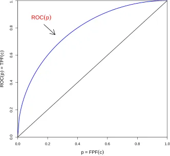
The receiver operating characteristic, or the ROC curve simply, has been
ex-tensively used to evaluate the diagnostic tests and is currently the best-developed
statistical tool for describing the performance of such tests. ROC curves provide a
comprehensive and visually attractive way to summarize the accuracy of predictions.
Generally speaking, the ROC curve is a graphical plot of the sensitivity, or true
positives, versus (1−specif icity), or false positives. It has been in use for years,
which was first developed during World War II for signal detection. Its potential for
medical diagnostic testing was recognized as early as 1960, although it was in the
early 1980s that it became popular, especially in radiology (Pepe, 2003). Nowadays,
ROC curves enjoy broader applications in medicine (Shapiro, 1999).
In a medical test resulting in a continuous measurement T, the disease is
diag-nosed if T > t, for a given threshold t. Let D denote the disease status with
D=
1, diseased,
0, non-diseased
respectively, where T P F(t) = P r(T ≥ t|D = 1), F P F(t) = P r(T ≥t|D = 0). The
ROC curve is the entire set of possible true and false positive fractions attained by
dichotomizing T with different thresholds (Pepe, 2003). That is, the ROC curve is
ROC(·) = {(F P F(t), T P F(t)), t∈(−∞,∞)}.
When t increases, both F P F(t) and T P F(t) decrease. For extreme cases, when
t→ ∞, we can get lim
t→∞T P F(t) = 0 and limt→∞F P F(t) = 0. On the other hand, when t→ −∞, we have lim
t→−∞T P F(t) = 1 and limt→−∞F P F(t) = 1. Thus, the ROC curve is actually a monotone increasing function in the positive quadrant.
On the other hand, considering the results of a certain test in two populations,
diseased against non-disease, we will rarely observe a perfect separation between the
two groups.
Suppose the distribution function of T is F conditional on disease and G
condi-tional on non-disease. The ROC curve is defined as the graph (1−G(t); 1−F(t)) for
various values of the thresholdt, or in other words,sensitivityversus (1−specif icity),
power versus size for a test with critical region {T > t}.
Now we consider a specific test in two populations, one with disease and the
other without disease. At a fixed cut-off point or threshold t, the sensitivity and
specificity are defined as Se = P r(X ≥ t) and Sp = P r(Y < t), respectively. If
F(·) is the distribution function ofX andG(·) is the distribution function ofY , the
sensitivity and specificity can then be written asSe= 1−F(t) andSp=G(t). Then
given level q= (1−specif icity), the ROC curve can be represented by
∆ = 1−F(G−1(1−q)), f or 0< q <1,
where G−1 is the inverse function of G, i.e., G−1(q) =inf{t: G(t)≥q}.
1.2 Missing Data and Random Hot Deck Imputation
It is typically to assume that all the responses in the sample are available for
statistical inferences. In practical applications, however, this may not be true. Some
of the responses may not be obtained for many reasons such as that some sampled
units are not willing to provide certain information, some of the investigators failed
to gather the correct information, uncontrollable factors leaded loss of information
and so forth. As a matter of fact, missing responses happen in a regular base in mail
enquiries, medical studies, opinion polls, market research surveys and other scientific
experiments (Wang and Rao, 2002).
Consider the following simple random samples of incomplete data associated with
populations (x, δx) and (y, δy):
(xi, δxi), i= 1, ..., m; (yj, δyj), j = 1, ..., n,
where
δxi =
0 if xi is missing,
1 otherwise,
δyj =
0 if yj is missing,
0.0 0.2 0.4 0.6 0.8 1.0
0.0
0.2
0.4
0.6
0.8
1.0
p = FPF(c)
ROC
(
p
)
= TPF
(
c
)
[image:14.612.134.466.255.559.2]ROC
(
p)
Let rx = m
X
1
δxi, ry =
n
X
1
δyj, mx = m−rx and my = n−ry. Denote the sets of
respondents with respect to x and y as srx and sry, and the sets of non-respondents
with respect to x and y as smx and smy, thus the means of respondents with respect
tox and y as
xr =
1 rx
X
i∈srx
xi, yr =
1 ry
X
i∈sry yi.
Throughout this thesis, we assume that x, y are missing completely at random
(M-CAR), i.e., P(δx = 1|x) = P1(constant) and P(δy = 1|y) = P2(constant). We also
assume that (x, δx) and (y, δy) are independent.
Imputation-based procedure is one of the most common methods or treatments
dealing with missing data (Little and Rubin, 2002). Standard statistics methods to
the complete data are applied after imputation, that is, to impute a value for each
missing datum. Deterministic imputation and random imputation are commonly used
imputation methods.
Here random hot deck imputation method is utilized to impute the missing
val-ues, since the deterministic imputation is not proper in making inference for
distri-bution functions.
Let x∗i and yj∗ be the imputed values for the missing data with respect to x
and y. Random hot deck imputation selects a simple random sample of size mx with
replacement fromsrx and then uses the associated x-values as donors, that is,x ∗
i =xk
for some k ∈srx. Similarly, we obtain y ∗
j. Let
xI,i =δxixi+ (1−δxi)x ∗
i, yI,j =δyjyj + (1−δyj)y ∗
j,
i= 1, ..., m, j = 1, ..., n, which represent the ’complete’ data after imputation.
ratio statistic for ∆ based on xI,i, i= 1, ..., m, yI,j, j = 1, ..., n. The results are used
to build asymptotic confidence intervals for ∆.
1.3 Empirical Likelihood
Empirical likelihood, a nonparametric method of statistical inference, use
like-lihood methods without having to assume that the data come from a known family
of distributions (Owen, 2001). Thus, empirical likelihood can be thought of as a
likelihood without parametric assumptions, and as a bootstrap without resampling.
Among many of the advantages over competitors, improvement of the confidence
re-gion and increase of accuracy in coverage are the most appealing features resulting
from using auxiliary information and easy implementation.
For a random variable X ∈ <, the cumulative distribution function (CDF) is
defined as
F(x) =P r(X ≤x),
where −∞< x <∞.
Denote
F(x−) =P r(X < x),
then
P r(X =x) = F(x)−F(x−).
LetX1, ..., Xnbe n independent samples follow the common CDF ofF0, the empirical
likelihood cumulative distribution function (ECDF) of X1, ..., Xn is defined as
Fn(x) =
1 n
n
X
i=1
where IXi≤x is the indicator function.
ForX1, ..., Xn,Xii.i.d.∼F0,i= 1, ..., n, the nonparametric likelihood of the CDF F
is
L(F) =
n
Y
i=1
(F(xi)−F(xi−)).
For a distribution F, ratios of the nonparametric likelihood for hypothesis testings
and confidence intervals is
R(F) = L(F) L(Fn)
.
When F is continuous, the likelihood of F, L(F)≡0. Owen (2001) also proves that
given F(x)6=Fn(x),
L(F)< L(Fn),
which means the ECDF is the nonparametric maximum likelihood estimate (NPMLE)
of F.
Suppose Γ is the space of a distribution functionG defined on [0,∞). ForF ∈Γ, let
θ =G(F), the profile likelihood ratio is defined as:
R(θ) = sup{R(F)|G(F) =θ, F ∈Γ}.
Then Owen (1990) gives a remarkable result similar to the Wilk’s theorem (Owen,
1988, 1990, 2001), that is, the empirical likelihood ratio has a limiting chi-square
distribution, as following:
−2 logR(θ0)→χ2m, as n→ ∞,
where m is the degrees of freedom d.f. = dimension(θ), θ0 is the true value of θ.
1.4 Structure
The rest of the thesis is organized as follows. In chapter 2, the empirical likelihood
ratio statistic is constructed, the limiting distribution of the statistic is given, and the
empirical likelihood based confidence interval for the cut-off points on the ROC curve
is constructed. In chapter 3, we report that the results of a simulation study on the
finite sample performance of empirical likelihood based confidence interval on ∆’s.
The conclusion is given in chapter 4, and all the technical derivations are provided in
Chapter 2
INFERENCE PROCEDURE
In this chapter, we construct the empirical likelihood ratio statistic, develop the
limiting distribution of the statistic, and give the empirical likelihood based confidence
interval for the ROC curve ∆.
Take the bandwidth a =am > 0,b =bn >0 and the kernelsK1 and K2, where
am →0 as m → ∞and bn→0 as n → ∞. Define
F(t) =
Z t/a
−∞
K1(u)du, G(t) =
Z t/b
−∞
K2(u)du.
Similar to Qin and Zhao (1997) and Chen and Hall (1993), the empirical likelihood
function is defined as
m Y i=1 pi n Y j=1
qj, (2.1)
where pi > 0, i=1,...,m,
X
i
pi = 1, and qj > 0, j=1,...,n,
X
j
qj = 1. Define the
log-empirical likelihood ratio statistic:
R(∆) = sup
pi,i=1,...,m,qj,j=1,...,n,θ {
m
X
i=1
log(mpi) + n
X
j=1
log(nqj)}= sup θ
where
R(∆, θ) = sup
pi,i=1,...,m,qj,j=1,...,n, {
m
X
i=1
log(mpi) + n
X
j=1
log(nqj)}, (2.3)
and pi, qj are subject to restrictions:
m
X
i=1
pi = 1, m
X
i=1
piF(θ−xI,i) = 1−∆, pi >0, i= 1, ..., m, (2.4)
and
n
X
j=1
qj = 1, n
X
j=1
qjG(θ−yI,j) = 1−q, qj >0, j = 1, ..., n. (2.5)
Denote
ω1(xI,i, θ,∆) =F(θ−xI,i)−1 + ∆, i= 1, ..., m,
ω2(yI,j, θ,∆) =G(θ−yI,j)−1 +q, j = 1, ..., n.
From Lagrange multipliers, we can show that
R(∆, θ) = −
m
X
i=1
log{1 +λ1(θ)ω1(xI,i, θ,∆)} − n
X
j=1
log{1 +λ2(θ)ω2(yI,j, θ,∆)}, (2.6)
where λj(θ), j = 1,2, are determined by the following two equations:
1 m
m
X
i=1
ω1(xI,i, θ,∆)
1 +λ1(θ)ω1(xI,i, θ,∆)
= 0, (2.7)
1 n
n
X
j=1
ω2(yI,j, θ,∆)
1 +λ2(θ)ω2(yI,j, θ,∆)
= 0. (2.8)
Let∂R(θ,∆)/∂θ= 0.We can obtain the empirical likelihood equation:
1 mλ1(θ)
m
X
i=1
α1(xI,i, θ,∆)
1 +λ1(θ)ω1(xI,i, θ,∆)
+ 1 mλ2(θ)
n
X
j=1
α2(yI,j, θ,∆)
1 +λ2(θ)ω2(yI,j, θ,∆)
where α1(xI,i, θ,∆) =
1
aK1((θ−xI,i)/a) and α2(yI,j, θ,∆) = 1
bK2((θ−yI,j)/b). Use θ0 to denote the true value ofθ, we have the following assumptions:
(i)θ0 ∈Ω and Ω is an open interval.
(ii) Denote f(t) = ∂F(t)/∂t and g(t) = ∂G(t)/∂t. For some t0 ≥ 2, suppose that
f(t0−1)(t) and g(t0−1)(t) exist and are uniformly continuous and bounded in a
neigh-borhood of θ0. Assume that f(θ0)g(θ0)>0.
(iii) n/m→k(0< k <∞) as m, n→ ∞.
(iv) For Ki’s, i = 1,2, are bounded and satisfy Lipschitz condition of order 1 and
Ki(2) exists and is bounded. For i= 1,2, assume that for some C >0,
Z
|u|>C/at0
K1(u)du=O(at0),
Z
|u|>C/bt0
K2(u)du=O(bt0),
Z
|ut0K
i(u)|du <∞,
Z
ujKi(u)du=
1 j = 0,
0 1≤j ≤t0−1.
(v) There exists r(1/3 < r < 1/2) such that nrat0 → 0, nrbt0 → 0, nra → ∞, and
nrb → ∞as m, n→ ∞.
Theorem 1 gives the asymptotic distribution of the log-empirical likelihood ratio
statistic. The proof of Theorem 1 is given in the Appendix A.
as m, n→ ∞,
√
m(θm,n −θ0)
d
− →
N
0, q(1−q)∆(1−∆){q(1−q)(1−P1+P −1
1 )f2(θ0) +k∆(1−∆)(1−P2+P2−1)g2(θ0)}
c2 0
,
−R(∆, θm,n) d
−
→ k∆(1−∆)(1−P1+P −1
1 )g2(θ0) +q(1−q)(1−P2+P2−1)f2(θ0)
c0
χ21,
where
c0 =q(1−q)f2(θ0) +k∆(1−∆)g2(θ0).
It is interesting to notice that the empirical likelihood ratio under imputation
is asymptotically distributed as a scaled chi-square variable. The reason for this
deviation from the standard results is that the ’complete’ data after imputation are
dependent.
Denote
a0(∆) ={k∆(1−∆)(1−P1+P1−1)g 2
(θ0) +q(1−q)(1−P2+P2−1)f 2
(θ0)}/c0.
To construct a confidence interval for ∆ using the above result, we need to get a
consistent estimator of a0(∆). P1 and P2 can be consistently estimated by
ˆ P1 =
1 m
m
X
i=1
δxi
and
ˆ P2 =
1 n
n
X
j=1
δyj,
respectively, and k is estimated by n/m. Similar to the proof of Lemma 2 in the
be shown that,
ˆ f(θ0) =
1 ma
m
X
i=1
K1((θm,n−xI,i)/a)
and
ˆ g(θ0) =
1 nb
n
X
j=1
K2((θm,n −yI,j)/b)
are consistent estimators of f(θ0) and g(θ0), respectively. In this case, we can get a
consistent estimator ˆa0(∆) of a0(∆).
Let tα satisfy that P(χ21 < tα) = 1−α. Thus, it follows from Theorem 1 that
the empirical likelihood based confidence interval for ∆ can be constructed as
{∆ : −2ˆa−01(∆)R(∆, θm,n)≤tα},
where the asymptotically correct coverage probability is 1−α.
We also notice that the result can apply to the complete data settings. In the
complete data situation, P1 = P2 = 1. Thus we can see that the asymptotic
distri-bution of the EL statistic is found to be a χ2
1 distribution. The empirical likelihood
based confidence interval for ∆ for the complete data is constructed as
Chapter 3
NUMERICAL STUDIES
3.1 Monte Carlo Simulation
Based on the results in the inference procedure, extensive simulation studies are
conducted to explore the performance of the empirical likelihood confidence intervals
for the ROC curve ∆, with different response rates and sample sizes.
In the simulation studies, the diseased population X is distributed as normal
distribution with mean 1 and variance 1, while the non-diseased populationY follows
the standard normal distribution. Random samplesxandyare independently drawn
from the populationXandY. The response rates forxandyare chosen as, (p1, p2) =
(0.7,0.6), (0.8,0.7), (0.9,0.8), combined with the sample sizes forxandy of (m, n) =
(50,50), (75,75), (100,100), (200,150). For a certain response rate and sample size,
1000 independent random samples of data {(xi, δxi), i= 1, ..., m; (yj, δyj), j = 1, ..., n}
are generated. Without loss of generality, the proposed empirical likelihood confidence
intervals are constructed for the ROC curve atq = 0.1, 0.3, 0.5, and0.7. The nominal
level of the confidence intervals is 1−α= 95%.
Tables 1 to 4 reveal the following results:
1. For each response rate and sample size, the coverage probability is close to the
nominal level 95%, and the average lengths of the confidence intervals are short.
the coverage probabilities get closer to 95%, and the average lengths of the intervals
decreases respectively. This is reasonable since either bigger response rates or bigger
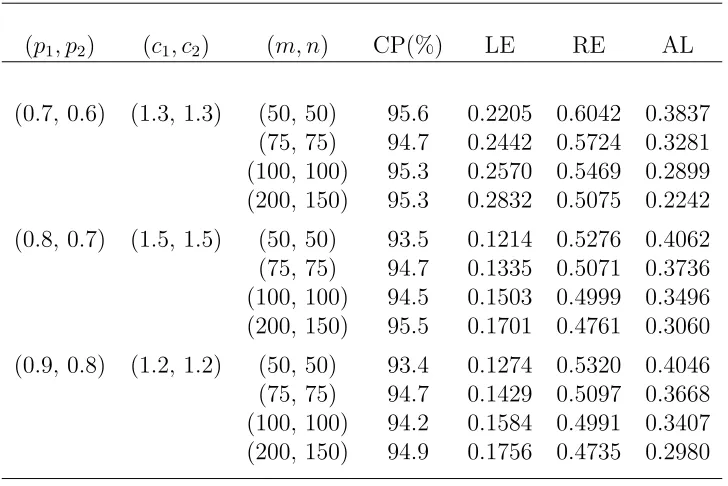
Table 3.1. Empirical likelihood confidence intervals for the ROC curve at q = 0.1 (∆ = 0.3891).
(p1, p2) (c1, c2) (m, n) CP(%) LE RE AL
(0.7, 0.6) (1.3, 1.3) (50, 50) 95.6 0.2205 0.6042 0.3837 (75, 75) 94.7 0.2442 0.5724 0.3281 (100, 100) 95.3 0.2570 0.5469 0.2899 (200, 150) 95.3 0.2832 0.5075 0.2242
(0.8, 0.7) (1.5, 1.5) (50, 50) 93.5 0.1214 0.5276 0.4062 (75, 75) 94.7 0.1335 0.5071 0.3736 (100, 100) 94.5 0.1503 0.4999 0.3496 (200, 150) 95.5 0.1701 0.4761 0.3060
(0.9, 0.8) (1.2, 1.2) (50, 50) 93.4 0.1274 0.5320 0.4046 (75, 75) 94.7 0.1429 0.5097 0.3668 (100, 100) 94.2 0.1584 0.4991 0.3407 (200, 150) 94.9 0.1756 0.4735 0.2980
NOTE:
CP(%): coverage probability, LE: the average left endpoint, RE: the average right endpoint
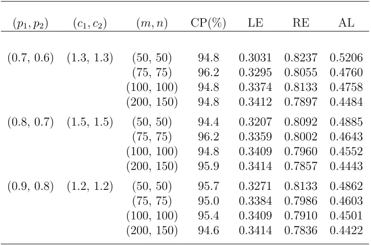
Table 3.2. Empirical likelihood confidence intervals for the ROC curve at q = 0.3 (∆ = 0.6828).
(p1, p2) (c1, c2) (m, n) CP(%) LE RE AL
(0.7, 0.6) (1.3, 1.3) (50, 50) 94.8 0.3031 0.8237 0.5206 (75, 75) 96.2 0.3295 0.8055 0.4760 (100, 100) 94.8 0.3374 0.8133 0.4758 (200, 150) 94.8 0.3412 0.7897 0.4484
(0.8, 0.7) (1.5, 1.5) (50, 50) 94.4 0.3207 0.8092 0.4885 (75, 75) 96.2 0.3359 0.8002 0.4643 (100, 100) 94.8 0.3409 0.7960 0.4552 (200, 150) 95.9 0.3414 0.7857 0.4443
(0.9, 0.8) (1.2, 1.2) (50, 50) 95.7 0.3271 0.8133 0.4862 (75, 75) 95.0 0.3384 0.7986 0.4603 (100, 100) 95.4 0.3409 0.7910 0.4501 (200, 150) 94.6 0.3414 0.7836 0.4422
NOTE:
CP(%): coverage probability, LE: the average left endpoint, RE: the average right endpoint
Table 3.3. Empirical likelihood confidence intervals for the ROC curve at q = 0.5 (∆ = 0.8413).
(p1, p2) (c1, c2) (m, n) CP(%) LE RE AL
(0.7, 0.6) (1.3, 1.3) (50, 50) 95.5 0.4167 0.9285 0.5118 (75, 75) 95.2 0.4202 0.9166 0.4964 (100, 100) 94.4 0.4207 0.9110 0.4903 (200, 150) 95.0 0.4207 0.8986 0.4780
(0.8, 0.7) (1.5, 1.5) (50, 50) 94.5 0.4204 0.9213 0.5009 (75, 75) 94.5 0.4207 0.9110 0.4903 (100, 100) 95.3 0.4207 0.9037 0.4831 (200, 150) 96.4 0.4207 0.8917 0.4710
(0.9, 0.8) (1.2, 1.2) (50, 50) 95.8 0.4205 0.9186 0.4981 (75, 75) 94.1 0.4207 0.9092 0.4885 (100, 100) 95.0 0.4207 0.9043 0.4836 (200, 150) 95.1 0.4207 0.8933 0.4726
NOTE:
CP(%): coverage probability, LE: the average left endpoint, RE: the average right endpoint
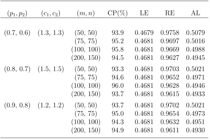
Table 3.4. Empirical likelihood confidence intervals for the ROC curve at q = 0.7 (∆ = 0.9363).
(p1, p2) (c1, c2) (m, n) CP(%) LE RE AL
(0.7, 0.6) (1.3, 1.3) (50, 50) 93.9 0.4679 0.9758 0.5079 (75, 75) 95.2 0.4681 0.9697 0.5016 (100, 100) 95.8 0.4681 0.9669 0.4988 (200, 150) 94.5 0.4681 0.9627 0.4945
(0.8, 0.7) (1.5, 1.5) (50, 50) 93.3 0.4681 0.9703 0.5021 (75, 75) 94.6 0.4681 0.9652 0.4971 (100, 100) 96.0 0.4681 0.9628 0.4946 (200, 150) 93.7 0.4681 0.9615 0.4933
(0.9, 0.8) (1.2, 1.2) (50, 50) 93.7 0.4681 0.9702 0.5021 (75, 75) 95.0 0.4681 0.9654 0.4973 (100, 100) 94.3 0.4681 0.9632 0.4951 (200, 150) 94.9 0.4681 0.9611 0.4930
NOTE:
CP(%): coverage probability, LE: the average left endpoint, RE: the average right endpoint
Chapter 4
SUMMARY AND FUTURE WORK
4.1 Summary
In this thesis, a smoothed empirical likelihood method is proposed to construct
the confidence intervals for ROC curves with missing data in both populations.
First, random hot deck imputation is applied to deal with data missing
complete-ly at random (MCAR). Then the empirical likelihood ratio statistic under imputation
can be proved to converge to a weighted chi-square distribution asymptotically. Then
the simulation studies evaluate the finite sample numerical performance of the
in-ference. All coverage probabilities are close to the nominal level of 95%, and larger
sample sizes lead to more accurate coverage probabilities, that is, closer to 95%,
and smaller average length of the confidence intervals as well. Moreover, when the
response rates are P1 = P2 = 1, which means both populations are complete, the
asymptotic limit distribution is reduced toχ2
1 distribution.
4.2 Future Work
In the future, we can continue the study in more than one way.
First, real data sets can be applied to testify the performance of the proposed
boot-strap method to explore better bandwidths for the kernel functions. Third, other
than the hot deck imputation used in the this thesis, we can try other imputation
methods, in order to utilize more information in the data.
In summary, the comparison of ROC curves can be further investigated in many
REFERENCES
[1] Chen, J. and Rao, J. N. K., Asymptotic normality under two-phase sampling designs, Statistica Sinica, Vol. 17, pp. 1047-1064, 2007.
[2] Chen, S. X., On the accuracy of empirical likelihood confidence regions for linear regression model, Annals of the Institute of Statistical Mathematics, Vol. 45, pp. 621-637, 1993.
[3] Chen, S. X., Empirical likelihood confidence intervals for linear regression coef-ficients, Journal of Multivariate Analysis, Vol. 49, pp. 24-40, 1994.
[4] Chen, S. X. and Hall, P., Smoothed empirical likelihood confidence intervals for quantiles, The Annals of Statistics, Vol. 21, pp 1166-1181, 1993.
[5] Chen, S. X. and Qin, J., Empirical likelihood-based confidence intervals for data with possible zero observations, Statistics & Probability Letters, Vol. 65, pp. 29-37, 2003.
[6] Claeskens, G., Jing, B.-Y., Peng, L. and Zhou, W., Empirical likelihood con-fidence regions for comparison distributions and ROC curves, The Canadian Journal of Statistics / La Revue Canadienne de Statistique, Vol. 31, pp. 173-190, 2003.
[7] DiCiccio, T., Hall, P. and Romano, J., Empirical likelihood is Bartlettcorrectable,
The Annals of Statistics, Vol. 19, pp. 1053-1061, 1991.
[8] Gastwirth, J. L. and Wang, J.-L., Control percentile test procedures for censored data, Journal of Statistical Planning and Inference, Vol. 18, pp. 267-276, 1988.
[9] Goddard, M. J. and Hinberg, I., Receiver operator characteristic (ROC) curves and non-normal data: An empirical study, Statistics in Medicine, Vol. 9, pp. 325-337, 1990.
[10] Hall, P. and La Scala, B., Methodology and algorithms of empirical likelihood,
International Statistical Review, Vol. 58, pp. 109-127, 1990.
[11] Hartley, H. O. and Rao, J. N. K., A new estimation theory for sample surveys,
Biometrika, Vol. 55, pp. 547-557, 1968.
[13] Li, G., Tiwari, R. C. and Wells, M. T., Quantile comparison functions in twosam-ple problems with application to comparisons of diagnostic markers, Journal of the American Statistical Association, Vol. 91, pp. 689-698, 1996.
[14] Liang, H. and Zhou, Y., Semiparametirc inference for ROC curves with censoring,
Scandinavian Journal of Statistics, Vol. 35, pp. 212-227, 2008.
[15] Little, R. J. A. and Rubin, D. B., Statistical Analysis with Missing Data, Wiley & JohnSons, 2nd edn.
[16] Lloyd, C. J. , Using smoothed receiver operating characteristic curves to sum-marize and compare diagnostic systems, Journal of the American Statistical As-sociation, Vol. 93, pp. 1356-1364, 1998.
[17] Owen, A.B., Empirical likelihood ratio confidence intervals for a single functional,
Biometrika, Vol. 75, pp. 237-249, 1988.
[18] Owen, A.B., Empirical likelihood ratio confidence regions. The Annals of Statis-tics, Biometrika, Vol. 18, pp. 90-120, 1990.
[19] Owen, A.B., confidence regions,Empirical likelihood, Chapman & Hall Ltd, 2001.
[20] Pepe, M. S., The Statistical Evaluation of Medical Tests for Classification and Prediction, Oxford: Oxford University Press.
[21] Qin, J., Empirical likelihood ratio based confidence intervals for mixture propor-tions, The Annals of Statistics, Vol. 27, pp. 1368-1384, 1999.
[22] Qin, J. and Lawless, J., Empirical likelihood and general estimating equations,
The Annals of Statistics, Vol. 22, pp. 300-325, 1994.
[23] Shapiro, D. E., The interpretation of diagnostic tests, Statistical Methods in Medical Research, Vol. 8, pp. 113-134, 1999.
[24] Su, H., Qin, Y. and Liang, H., Empirical Likelihood-Based Confidence Interval of ROC Curves, Statistics in Biopharmaceutical Research, Vol. 1, pp. 407-414, 2009.
[25] Thomas, D. R. and Grunkemeier, G. L., Confidence interval estimation of sur-vival probabilities for censored data,Journal of the American Statistical Associ-ation, Vol. 70, pp. 865-871, 1975.
[26] Tosteson, A. A. N. and Begg, C. B., A general regression methodology for roc curve estimation, Medical Decision Making, Vol. 8, pp. 204-215, 1988.
[28] Zhou, W. and Jing, B.-Y., Smoothed empirical likelihood confidence intervals for the difference of quantiles, Statistica Sinica, Vol. 13, pp. 83-95, 2003.
[29] Zhou, X.-H., McClish, D. K. and Obuchowski, N. A., Statistical Methods in Diagnostic Medicine, Wiley.
[30] Zhou, Y. and Liang, H., Empirical-likelihood-based semiparametric inference for the treatment effect in the two-sample problem with censoring, Biometrika, Vol. 92, pp. 271-282, 2005.
[31] Zou, K. H., Hall, W. J. and Shapiro, D. E. , Smooth non-parametric receiver operating characteristic (ROC) curves for continuous diagnostic tests, Statistics in Medicine, Vol. 16, pp. 2143-2156, 1997.
APPENDICES
Appendix A: Lemmas and Proofs
The following lemma of Chen and Rao (2007) will be used later.
Lemma 1. LetUn, Vnbe two sequences of random variables and letBn be aσ-algebra.
Assume that
1. There exists σ1n >0 such that
σ1−n1Vn d
−
→N(0,1),
as n→ ∞, where Vn is Bn measurable.
2. E[Un|Bn] = 0 and V ar(Un|Bn) =σ22n such that
sup
t
|P(σ2−n1Un≤t|Bn)−Φ(t)|=op(1),
where Φ(.) is the distribution function of the standard normal random variable.
3. γ2
n=σ21n/σ22n=γ2+op(1)
Then, as n→ ∞,
Un+Vn
p
σ2
1n+σ22n d
−
→N(0,1).
Lemma 2. Under the conditions of Theorem 1, as m, n→ ∞, we have 1 √ m m X i=1
ω1(xI,i, θ0,∆)
d
−
→N(0, σ12),
1 √ n n X i=1
ω2(xI,i, θ0,∆)
d
−
→N(0, σ22),
and 1 m m X i=1
ω12(xI,i, θ0,∆) = ∆(1−∆) +op(1),
1 n
n
X
i=1
ω22(yI,j, θ0,∆) =q(1−q) +op(1),
where
σ21 = (1−P1+P1−1)∆(1−∆), σ 2
2 = (1−P2+P2−1)q(1−q).
Proof of Lemma 2. Letω1r =
1 rx
X
i∈Srx
ω1(xi, θ0,∆) and Bm =σ((δxi, xi), i= 1, ..., m).
Then
E(ω1(x∗i, θ0,∆)|Bm) =ω1r,
V ar(ω1(x∗i, θ0,∆)|Bm) =
1 rx
X
i∈Srx
{ω1(xi, θ0,∆)−ω1r}2.
It follows that
1 √ m m X i=1
ω1(xI,i, θ0,∆) =
√
mω1r+
1 √
m
X
i∈Smx
{ω1(x∗i, θ0,∆)−E(ω1(x∗i, θ0,∆)|Bm)}
=Vm+Um.
Vm is Bm measurable and
Vm=
√ m 1
rx
X
i∈Srx
{ω1(xi, θ0,∆)−Eω1(xi, θ0,∆)}+
√
mEω1(xi, θ0,∆).
It can be shown that Eω1(xi, θ0,∆) =O(at0). Thus from Assumption (iii) and (v), it
follows that √mEω1(xi, θ0,∆) = o(1). Combining with the MCAR assumption and
the Central Limit Theorem (CLT), it gives,
Vm d
−
→N(0, P1−1∆(1−∆)).
From Berry-Esseen’s Central Limit Theorem for independent random variables, we
have
sup
t
|P(σ2−m1Um ≤t|Bm)−Φ(t)|=op(1),
where σ2
2m = (1−P1)Eω1(x, θ0,∆) = (1−P1)∆(1−∆). Hence, from Lemma 1, we
have 1 √ m X i
ω1(xI,i, θ0,∆)
d
−
→N(0, σ12).
On the other hand, denote the conditional probability given Bm asP∗. Then by the
Law of Large Numbers and MCAR assumption,
1 mx
X
i∈smx
ω12(x∗i, θ0,∆) =
1 rx
X
i∈srx
ω12(xi, θ0,∆) +oP∗(1) =Eω2
It follows that 1 m m X i=1
ω12(xI,i, θ0,∆) =
1 m
m
X
i=1
{δxiω12(xi, θ0,∆) + (1−δxi)ω12(x
∗
i, θ0,∆)}
=P1Eω12(x, θ0,∆) +op(1) +
mx
m 1 mx
X
i∈smx
ω12(x∗i, θ0,∆)
= 1
m
m
X
i=1
{δxiω12(xi, θ0,∆) + (1−δxi)ω12(x
∗
i, θ0,∆)}
=P1Eω12(x, θ0,∆) +op(1) + (1−P1)Eω12(x, θ0,∆) +op(1)
=Eω21(x, θ0,∆) +op(1)
= ∆(1−∆) +op(1).
The rest of Lemma 2 can be proved similarly. So the proof of Lemma 2 is complete.
Lemma 3. Suppose that1/3< η <1/2and the conditions of Theorem 1 are satisfied. Then, as m, n→ ∞,
λ1(θ) = Op(n−ηa−1+at0),
and
λ2(θ) = Op(n−ηb−1+bt0),
uniformly about θ∈ {θ :|θ−θ0| ≤cn−η}, where c is a positive constant.
Proof of Lemma 3. It can be shown that
|ω1(xI,i, θ,∆)−ω1(xI,i, θ0,∆)| ≤ca−1n−η
for some constant cas θ∈ {θ :|θ−θ0| ≤cn−η}. Combining with Lemma 2 we have
1 m
m
X
i=1
1 m
m
X
i=1
ω12(xI,i, θ,∆) = ∆(1−∆) +op(1).
Denote Zm = max
1≤i≤m|ω1(xI,i, θ,∆)|. Then Zm ≤c, a.s.Thus equation (2.7) gives that
|λ1(θ)|
1 +Zm|λ1(θ)|
{∆(1−∆) +OP(1)}=Op(n−ηa−1+at0).
Thereforeλ1(θ) =Op(n−ηa−1+at0). The rest of Lemma 2 can be proved similarly.
Lemma 4. Suppose that1/3< η <1/2and the conditions of Theorem 1 are satisfied. Then with probability tending to 1 there exists a root θm,n of equation (2.9) such that,
as m, n→ ∞,
|θm,n−θ0|=Op(n−η),
and R(∆, θ) attains its local maximum value at θm,n.
Proof of Lemma 4. Take |θ − θ0| = n−η. Denote ω1j(θ) =
1 m
m
X
i=1
ω1j(xI,i, θ,∆) for
j = 1, 2 and
R1(∆, θ) = −
m
X
i=1
log{1 +λ1(θ)ω1(xI,i, θ,∆)},
R2(∆, θ) = −
n
X
j=1
log{1 +λ2(θ)ω2(yI,j, θ,∆)}.
From equation (2.7), we obtain that
ω11(θ)−λ1(θ)ω12(θ) +
1 mλ
2 1(θ)
m
X
i=1
ω3
1(xI,i, θ,∆)
1 +λ1ω1(xI,i, θ,∆)
= 0.
Using Lemma 3, we have
By the Taylor expansion we have
−R1(∆, θ) =
m
X
i=1
λ1(θ)ω1(xI,i, θ,∆)−
1 2
m
X
i=1
λ21(θ)ω12(xI,i, θ,∆) +Op{mλ31(θ)}
=mλ1(θ)ω11(θ)−
1 2mλ
2
1(θ)ω12(θ) +Op{mλ31(θ)}
= m
2{ω12(θ)} −1{
ω11(θ)}2+Op{mλ31(θ)}
= m
2{ω12(θ0) + 0p(1)} −1{ω
11(θ0) +γ11(θ0)n−η +Op(n−2η)}2+Op{mλ31(θ)}
= m
2{q(1−q) + 0p(1)} −1{ω
11(θ0) +f(θ0)n−η +op(n−η)}2+op(mm−2η),
where γ11(θ0) = ma1
X
i
K((θ0−xI,i)/a). From Assumptions (iii), (v), Lemma 3 and
its proof, it follows thatω11(θ0) =Op(at0 +m−1/2) =op(m−η). Thus,
−R1(∆, θ) =
m
2{q(1−q)}
−1+f2(θ
0)n−2η +op(mn−2η).
On the other hand, from the above derivations, we can see that
−R1(∆, θ) = op(mn−2η).
It follows that, when|θ−θ0|=n−η, with probability tending to 1,
−R1(∆, θ)>−R1(∆, θ0).
Similarly,
−R2(∆, θ)>−R2(∆, θ0).
Thus,
From the continuity of R(∆, θ), we have Lemma 4.
Lemma 5. Suppose that the conditions of Theorem 1 are satisfied and that θm,n is
as in Lemma 4. Then, as m, n→ ∞,
√
m(θm,n−θ0)
d
−
→N(0,(f2(θ0)σ21+kg 2(θ
0+ ∆)σ22)/c 2 0),
λ1(θm,n) =−
kg(θ0+ ∆)
f(θ0)
λ29θm,n) +op(n−1/2),
√
mλ2(θm,n) d
−
→N(0, σ2),
where
σ2 ={q(1−q)}−1f2(θ 0)
(1−P1+P1−1)g2(θ0+ ∆) +k−1(1−P2 +P2−1)f2(θ0)
c20 ,
and σj2, j = 1,2 and c0 are defined as in Lemma 2 and Theorem 1.
Proof of Lemma 5. Letλ1 =λ1(θ), λE1 =λ1(θm,n), λ2 =λ2(θ), λE2 =λ2(θm,n) and
Q1,m,n(θ, λ1, λ2) =
1 m
m
X
i=1
ω1(xI,i, θ,∆)
1 +λ1ω1(xI,i, θ,∆)
,
Q2,m,n(θ, λ1, λ2) =
1 n
n
X
j=1
ω2(yI,j, θ,∆)
1 +λ2ω2(yI,j, θ,∆)
,
Q3,m,n(θ, λ1, λ2) =
λ1
ma
m
X
i=1
K1((θ−xI,i)/a)
1 +λ1ω1(xI,i, θ,∆)
+ λ2 mb
n
X
j=1
K2((θ−yI,j)/b)
1 +λ2ω2(yI,j, θ,∆)
.
From Lemma 4, we have
From the Taylor expansion and Lemma 3 and Lemma 4, we have
0 = Qi,m,n(θm,n, λE1, λE2)
=Qi,m,n(θ0,0,0) +
∂Qi,m,n(θ0,0,0)
∂θ (θm,n−θ0) + ∂Qi,m,n(θ0,0,0)
∂λ1
λE1+
∂Qi,m,n(θ0,0,0)
∂λ2
λE2+op(n), i= 1,2,3,
where n=|θm,n−θ0|+|λE1|+|λE2|. Hence
Qi,m,n(θ0,0,0) +
∂Qi,m,n(θ0,0,0)
∂θ (θm,n−θ0) +∂Qi,m,n(θ0,0,0)
∂λ1
λE1+
∂Qi,m,n(θ0,0,0)
∂λ2
λE2 =op(n), i= 1,2,3.
(2)
Similar to the proof of Lemma 2, it can be shown that
∂Q1,m,n(θ0,0,0)
∂θ =f(θ0) +op(1), ∂Q1,m,n(θ0,0,0)
∂λ1
=−∆(1−∆) +op(1),
∂Q1,m,n(θ0,0,0)
∂λ2
= 0,
∂Q2,m,n(θ0,0,0)
∂θ =g(θ0) +op(1), ∂Q2,m,n(θ0,0,0)
∂λ1
= 0,
∂Q2,m,n(θ0,0,0)
∂λ2
=−q(1−q) +op(1),
∂Q3,m,n(θ0,0,0)
∂θ = 0, ∂Q3,m,n(θ0,0,0)
∂λ1
=f(θ0) +op(1),
∂Q3,m,n(θ0,0,0)
∂λ2
Thus
θm,n−θ0
λE1
λE2
=S−1
−Q1,m,n(θ0,0,0)
−Q2,m,n(θ0,0,0)
0
+op(n),
where S =
f(θ0) −∆(1−∆) 0
g(θ0) 0 −q(1−q)
0 f(θ0) kg(θ0)
.
Combining with √nQj,m,n(θ0,0,0) = Op(1), j = 1,2, we have n = Op(n−1/2). It
follows that
θm,n−θ0 =−
1 c0
{q(1−q)f(θ0)Q1,m,n(θ0,0,0)+k∆(1−∆)g(θ0)Q2,m,n(θ0,0,0)}+op(n−1/2),
λE1 =
kg(θ0)
c0
{g(θ0)Q1,m,n(θ0,0,0)−f(θ0)Q2,m,n(θ0,0,0)}+op(n−1/2),
λE2 =−
f(θ0)
c0
{g(θ0)Q1,m,n(θ0,0,0)−f(θ0)Q2,m,n(θ0,0,0)}+op(n−1/2).
From Lemma 2, we have
√ m
Q1,m,n(θ0,0,0)
Q2,m,n(θ0,0,0)
d − →N 0,
σ21 0
0 k−1σ22
.
Thus Lemma 5 is proved.
shown that
−2R(∆, θm,n)
=mλ21(θm,n)×
1 m
m
X
i=1
ω12(xI,i, θ,∆) +nλ22(θm,n)×
1 n
n
X
j=1
ω22(yI,j, θ,∆) +op(1).