Assessing the performance of global hydrological models for capturing peak river flows in the Amazon basin

https://doi.org/10.5194/hess-23-3057-2019 © Author(s) 2019. This work is distributed under the Creative Commons Attribution 4.0 License.

Assessing the performance of global hydrological models

for capturing peak river flows in the Amazon basin

Jamie Towner1, Hannah L. Cloke1,2,4,5, Ervin Zsoter3,1, Zachary Flamig6, Jannis M. Hoch7,8, Juan Bazo10,11, Erin Coughlan de Perez9,10, and Elisabeth M. Stephens1

1_{Department of Geography & Environmental Science, University of Reading, Reading, RG6 6AB, UK} 2_{Department of Meteorology, University of Reading, Reading, RG6 6BB, UK}

3_{European Centre for Medium-Range Weather Forecasts, Shinfield Park, Reading, RG6 9AX, UK} 4_{Department of Earth Sciences, Uppsala University, Uppsala, 752 36, Sweden}

5_{Centre of Natural Hazards and Disaster Science, CNDS, Uppsala, 752 36, Sweden} 6_{University of Chicago Center for Data Intensive Science, Chicago, USA}

7_{Department of Physical Geography, Utrecht University, P.O. Box 80115, 3508 TC Utrecht, the Netherlands} 8_{Deltares, P.O. Box 177, 2600 MH Delft, the Netherlands}

9_{International Research Institute for Climate and Society, Columbia University, Palisades, NY 10964, USA} 10_{Red Cross Red Crescent Climate Centre, 2521 CV The Hague, the Netherlands}

11_{Universidad Tecnológica del Perú (UTP), Lima, Peru} Correspondence:Jamie Towner ([email protected]) Received: 29 January 2019 – Discussion started: 27 February 2019 Revised: 8 June 2019 – Accepted: 26 June 2019 – Published: 18 July 2019

Abstract.Extreme flooding impacts millions of people that live within the Amazon floodplain. Global hydrological mod-els (GHMs) are frequently used to assess and inform the management of flood risk, but knowledge on the skill of available models is required to inform their use and develop-ment. This paper presents an intercomparison of eight differ-ent GHMs freely available from collaborators of the Global Flood Partnership (GFP) for simulating floods in the Ama-zon basin. To gain insight into the strengths and shortcom-ings of each model, we assess their ability to reproduce daily and annual peak river flows against gauged observations at 75 hydrological stations over a 19-year period (1997–2015). As well as highlighting regional variability in the accuracy of simulated streamflow, these results indicate that (a) the me-teorological input is the dominant control on the accuracy of both daily and annual maximum river flows, and (b) ground-water and routing calibration of Lisflood based on daily river flows has no impact on the ability to simulate flood peaks for the chosen river basin. These findings have important rel-evance for applications of large-scale hydrological models, including analysis of the impact of climate variability, assess-ment of the influence of long-term changes such as land-use

and anthropogenic climate change, the assessment of flood likelihood, and for flood forecasting systems.

1 Introduction

agri-cultural and fishery practices (Schöngart and Junk, 2007; Marengo et al., 2012, 2013; Correa et al., 2017). Single flood events (e.g. 2012 in the Amazonian city of Iquitos, Peru) have impacted the lives of over 73 000 people (IFRC, 2013), with average annual damages estimated at USD 1.4 billion over a 4-year period (2008–2011) in the Brazilian Rio Branco basin alone (Mundial Grupo Banco, 2014).

1.1 Global hydrological models and applications In its simplest form, a hydrological model can be consid-ered a representation of a real-world hydrological system used to better understand various water and environmental processes, predict system behaviour, and provide consistent impact assessment (Devia et al., 2015). They work by simu-lating the hydrological response to meteorological variations incorporating run-off generation and river routing processes (Sutanudjaja et al., 2018). As such, global hydrological mod-els (GHMs) have been used in a wide range of applications, including short- to extended-range flood forecasting (Alfieri et al., 2013; Emerton et al., 2018), climate assessment (Hat-termann et al., 2017), hazard and risk-mapping (Ward et al., 2015), drought prediction (van Huijevoort et al., 2014), and water resource assessment (e.g. water availability models; Meigh et al., 1999; Sood and Smakhtin, 2015).

Depending on the application and the needs of decision makers, different properties of the hydrograph simulated by hydrological models are important. For example, an accurate representation of peak river flows and their likelihood is key for decision-makers who wish to understand the area at risk of flooding. In contrast, estimates of daily streamflow may be more beneficial for the assessment of water resources such as irrigation requirements.

1.2 GHM development

The availability of GHMs has grown in recent years thanks to increased efforts in addressing water-related issues in de-veloping countries (De Groeve et al., 2015; Ward et al., 2015; Trigg et al., 2016), the development of flood forecasting sys-tems (Aliferi et al., 2013; Werner et al., 2013; Emerton et al., 2018), improvements within precipitation datasets (Mitter-maier et al., 2013; Novak et al., 2014; Forbes et al., 2015), the emergence of new global satellite and remote sensing datasets, and advancements in numerical modelling tech-niques (Yamazaki et al., 2014a; Sampson et al., 2015; An-dreadis et al., 2017; Balsamo et al., 2018). For an overview of available GHMs, see Bierkens et al. (2015), who have pro-vided the details of 22 large-scale hydrological models, with those used for operational flood forecasting being summa-rized in Emerton et al. (2016).

1.3 Land surface models vs. hydrological models GHMs have differing spatial and temporal resolutions, pa-rameter estimation approaches, number of papa-rameters, cal-ibration methods, input–output variables, and overall struc-tures (Sood and Smakhtin, 2015). Their set-ups can generally be divided into two categories: land surface models (LSMs) and hydrological models (Gudmundsson et al., 2012). The majority of LSMs and hydrological models share the same conceptualization of the water balance (Haddeland et al., 2011) but differ in their objective. LSMs evolve from cou-pled land–atmosphere models with the purpose of solving the surface energy balance equations to provide the neces-sary lower boundary conditions to the atmosphere (Wood et al., 2011). In contrast, hydrological models tend to focus less on the partitioning of radiation and more on hydrological re-sources and understanding the lateral movement and trans-port of water along the land surface.

In terms of differences in model performance, the Gud-mundsson et al. (2012) intercomparison study of six LSMs and five GHMs (i.e. hydrological models) concluded that the main differences were due to the snow scheme implemented with snow water equivalent values and mean runoff fractions lower in LSMs. No significant differences between LSMs and hydrological models were found for runoff and evap-otranspiration globally, but rather the differences between the models themselves created large sources of uncertainty, highlighting the importance of analysing a range of differ-ent GHMs rather than a group consisting of a specific model type. For the purposes of this study, we categorize both LSM and hydrological models as GHMs.

1.4 Motivation

For GHMs to be considered effective, end users need to know their accuracy and reliability (Ward et al., 2015). Thus, the evaluation of these models against observed data is an im-portant procedure in efforts to reduce flood risk. Currently, no intercomparison analysis of GHMs has been conducted specifically for the Amazon basin, with previous studies fo-cusing solely on the performance of individual models for the Amazon (e.g. Yamazaki et al., 2012; Paiva et al., 2013; Hoch et al., 2017a, b) or as part of a global study (e.g. Gudmunds-son et al., 2012; Alfieri et al., 2013; Hirpa et al., 2018), which lack an in-depth focus on skill within the Amazon basin.

which exist within the model set-ups and help to distinguish how different parts of the hydrological chain can cause par-ticularly “good” or “bad” model performance, thus having implications for their different applications.

1.5 Objectives

In this study, the main objective is to assess the ability of different GHMs freely available from collaborators within the Global Flood Partnership (GFP), identifying which ap-proaches are most suitable in different areas of the Amazon basin for simulating flood peaks. To pursue this objective, the analysis is designed to answer the following research ques-tions.

1. How well do GHMs represent the annual hydrological regime in terms of the Kling–Gupta efficiency (KGE) and its individual components?

2. Which model set-up best represents annual maximum river flows?

3. Which hydrological routing model allows the best rep-resentation of daily and peak river flows?

4. Which precipitation dataset allows the best representa-tion of daily and peak river flows?

5. How do results differ when using a LSM as opposed to a hydrological model?

6. By how much does calibration of groundwater and rout-ing model parameters improve performance?

2 Data and methodology

The experimental design involves comparing the output of daily and annual maximum discharge estimates produced by different GHMs forced using atmospheric reanalysis or satel-lite precipitation datasets against observations of streamflow. The common validation period is 1997–2015, with results also analysed for the shorter period of 2004–2015 to account for the shorter record length of one simulation.

2.1 Observations

Observed daily discharge data are used to evaluate each of the model runs. The network of hydrometric gauges is con-trolled and maintained by the national institutions responsi-ble for hydrological monitoring in countries situated within the Amazon basin. These include the Agência Nacional de Águas (Water National Office – ANA, Brazil), Servicio Na-cional de Meteorología e Hidrología (National Meteorology and Hydrology Service – SENAMHI, Peru and Bolivia), Instituto Nacional Meteorologia e Hidrologia (Institute to Meteorology and Hydrology, INAMHI, Ecuador), and the

Instituto de Hidrología, Meteorología y Estudios Ambien-tales (Institute of Hydrology, Meteorology and Environmen-tal Studies – IDEAM, Colombia).

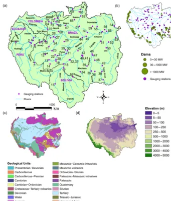
Daily water level values are collected by the respective institutions and are sourced through the ORE-HYBAM ob-servational service (http://www.ore-hybam.org/, last access: 1 December 2018), in collaboration with the Institute of Re-search for Development (IRD) or directly from the national services. A time series of daily river flow for each station is obtained using stage and rating curve measurements which were determined using an acoustic Doppler current pro-filer (ADCP) conducted by the ORE-HYBAM observatory and SENAMHI (Espinoza et al., 2014). In total 75 hydrolog-ical stations throughout the Amazon basin are selected, with an average record length of 17 years within the main valida-tion period (1997–2015). The locavalida-tions of stavalida-tions and their characteristics are displayed in Fig. 1a and Table S1 in the Supplement respectively. Stations selected have a minimum of 5 consecutive years’ worth of data during the main valida-tion period. The threshold was set to 5 to prevent the elimi-nation of stations in data-scarce areas such as Peru, Bolivia, and Colombia.

2.2 Routing models and meteorological datasets Eight GHMs composed of different meteorological datasets, hydrological models/LSMs, and river routing models are used to each simulate river discharge across the Amazon basin. Four meteorological products (ERA-Interim Land re-analysis, ERA-5 re-re-analysis, European Centre for Medium-range Weather Forecasts (ECMWF) 20-year control refore-casts (hereafter defined as reforerefore-casts), and the real-time TRMM TMPA 3B42 v.7), three hydrological models/LSMs (PCR-GLOBWB, the Hydrology-Tiled ECMWF Scheme for Surface Exchanges over Land; H-TESSEL, EF5), and three river routing models (Catchment-based Macro-scale Flood-plain model, CaMa-Flood; Lisflood; and the Coupled Rout-ing and Excess Storage, CREST) are employed. While the focus of this study is on GHMs made available by the GFP community, other models are available within the Amazon basin. Some examples include MGB-IPH (Paiva et al., 2013), LPJmL (Lund–Potsdam–Jena managed Land; Bondeau et al., 2007), WaterGAP (water – global analysis and progno-sis; Döll et al., 2003), and MAC-PDM.09 (the Macro-scale-Probability-Distributed Moisture model.09; Gosling and Ar-nell, 2011).

Figure 1. (a)Locations of the 75 hydrological gauges and the river network of the Amazon basin. Numbers represent stations which are

referred to throughout the main text in italics. For station information, see Table S1.(b)Locations of existing and under-construction dams

as of 2017 (see Latrubesse et al., 2017).(c)Geological map of the Amazon (Schenk et al., 1999).(d)Elevation map of the basin from the

digital elevation model (DEM), GTOPO30, at a horizontal resolution of approximately 1 km (US Geological Survey, 1996).

of Lisflood, whereby the routing and LSM remain consis-tent. To evaluate the differences between using the Lisflood and CaMa-Flood routing models, two simulations which use ERA-Interim Land precipitation and the H-TESSEL LSM are compared. To identify the differences between employ-ing a hydrological model (PCR-GLOBWB) or LSM (H-TESSEL), two set-ups which use the ERA-Interim Land precipitation reanalysis and the CaMa-Flood river routing model are directly compared. Finally, to see how much bene-fit model calibration within Lisflood provides, ERA-Interim Land and ERA-5 are forced through the calibrated and un-calibrated Lisflood model versions. The CREST EF5 run is the sole simulation to have a unique hydrological model and meteorological input, and although it is more challenging to analyse the performance of specific components of the model

set-up against other simulations, it was included in the anal-ysis for completeness.

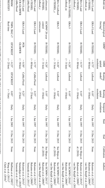
regarding the differences in skill. Finally, short descriptions of each model and atmospheric product are outlined below, with a summary of each simulation provided in Table 1.

2.2.1 Precipitation datasets

ERA-Interim Land is a global reanalysis of land surface parameters produced by the ECMWF with a T255 spec-tral resolution (∼80 km or∼0.75◦; Balsamo et al., 2015). ERA-Interim Land was produced using the latest version of the land surface H-TESSEL model using atmospheric forcing from ERA-Interim (Dee et al., 2011), with precip-itation adjustments based on the Global Precipprecip-itation Cli-mate Project (GPCP) v2.1. Precipitation improvements were achieved by Balsamo et al. (2010) using a scale-selective rescaling procedure in which ERA-Interim 3-hourly precipi-tation was corrected to match the monthly accumulation pro-vided by the GPCP at grid point scale (Huffman et al., 2009). All simulations which use ERA-Interim Land are run of-fline to force the associated rainfall–runoff models (see Ta-ble 1). For a detailed description of the ERA-Interim Land and ERA-Interim datasets, see Balsamo et al. (2015) and Dee et al. (2011) respectively. Dataset available at http://apps. ecmwf.int/datasets/data/interim-full-daily/levtype=sfc/ (last access: 1 July 2018).

ERA-5 is the latest reanalysis product of the ECMWF producing consistent estimates of atmospheric, land, and ocean variables at a horizontal resolution of∼31 km, while the vertical atmosphere is discretized into 137 levels to 0.01 hPa (ECMWF, 2018). ERA-5 is based on the Inte-grated Forecasting System (IFS) Cycle 41r2 which was used operationally at the ECMWF in 2016. Early analysis has shown that ERA-5 has an improved representation of precipitation (particularly over land in the deep tropics), evaporation, and soil moisture compared to its predecessor ERA-Interim Land (ECMWF, 2017). ERA-5 is currently being produced in three “streams” and will eventually cover the period 1950 to near real time (∼3 d) with its completion due in 2019 (Emerton et al., 2018). Dataset available at https://software.ecmwf.int/wiki/display/CKB/How+to+ download+ERA5+data+via+the+ECMWF+Web+API (last access: 1 July 2018).

ECMWF reforecasts are a collection of historical forecasts from start dates at the same day of the year going back for a specific number of years to provide a consistent model clima-tology from which to compare forecasts (ECMWF, 2016). In this study we use the control member of the reforecasts which are created based on a retrospective run of the most recent version of the ECMWF’s IFS to provide surface and subsurface runoff as input to the Lisflood routing model at a resolution of 0.1◦. The reforecast run is computed using a lighter configuration (11 ensemble members, run twice a week on Mondays and Thursdays) to reduce computational time. The purpose of running the ECMWF forecasts through the Lisflood routing model is to generate a long-term

(20-year) dataset which is consistent with operational GloFAS forecasts enabling the suitability of the dataset for use in the calibration of the Lisflood model parameters (Hirpa et al., 2018). These data cover the period June 1995 to June 2015 and due to frequent model updates of the IFS are based on multiple model cycles: Cycle 41r1 (July through to March) and Cycle 41r2 (March through to June). The control refore-casts from Mondays and Thursdays are used subsequently to fill the whole weeks by taking the first 3 and 4 d forecast periods respectively throughout the 20 years.

TRMM TMPA 3B42 RT v7 is a global merged multi-satellite precipitation product generated at the National Aero-nautics and Space Administration (NASA). TMPA is com-puted for two products: a near-real-time version (TMPA 3B42RT v7) and a post-real-time gauged adjusted research version (TMPA 3B42 v7), both of which run at resolu-tion of 3-hourly×0.25◦_×0.25◦_{(Huffman et al., 2007). The}

TMPA 3B42 RT gridded dataset used in this study covers the global latitude belt from 60◦N to 60◦S. For further in-formation, see Huffman et al. (2007). Dataset available at https://pmm.nasa.gov/data-access/downloads/trmm (last ac-cess: 4 March 2018).

2.2.2 Hydrological and land surface models

H-TESSEL provides the land surface component of the ECMWF IFS (van den Hurk et al., 2000; van den Hurk and Viterbo, 2003; Balsamo et al., 2009). H-TESSEL simulates the land surface response to atmospheric conditions estimat-ing water and energy fluxes (heat, moisture, and momen-tum) on the land surface (Zsoter et al., 2019). H-TESSEL is predominately used within the operational set-up of short-to seasonal-range weather forecasts coupled with the atmo-sphere, but it can also be used in an “offline mode” to calculate the land surface response to atmospheric forcing, whereby input data (e.g. near-surface meteorological condi-tions) are provided on a 3-hourly time step (Pappenberger et al., 2012). In this study, H-TESSEL receives boundary con-ditions from the atmospheric input provided by either the ERA-5 reanalysis, ERA-Interim Land reanalysis, or the re-forecasts providing total runoff for the CaMa-Flood routing model, and the surface and sub-surface water fluxes for Lis-flood. Runs forced using the ERA-Interim Land reanalysis are run in the offline mode. For a detailed description of H-TESSEL, see Balsamo et al. (2009).

network using the kinematic routing wave equation. PCR-GLOBWB was applied at a resolution of 30 arcmin (∼55 km ×55 km at the Equator) with meteorological forcing pro-vided from the ERA-Interim Land reanalysis dataset be-tween 1997 and 2015. For further information on PCR-GLOBWB, see van Beek and Bierkens (2008), van Beek et al. (2011), and Sutanudjaja et al. (2018).

EF5 is an open-source software package developed at the University of Oklahoma (OU) that consists of multiple hy-drological model cores producing outputs of streamflow, wa-ter depth, and soil moisture (Clark et al., 2016). Since 2016, EF5 has been used operationally for local forecasts across the US National Weather Service (NWS) for flash flooding purposes (Gourely et al., 2017). EF5 incorporates CREST, which is a distributed hydrological model created by OU and NASA (Wang et al., 2011). Within CREST, runoff genera-tion, evapotranspiragenera-tion, infiltragenera-tion, and surface and subsur-face routing are computed at each grid cell within the model domain, with surface and subsurface water routed using a kinematic wave assumption. Four excess storage reservoirs characterize the vertical profile within a cell representing in-terception by the vegetation canopy and subsurface water storage in the three soil layers (Meng et al., 2013). In ad-dition, the representation of sub-grid cell routing and soil moisture variability is made through the use of two linear reservoirs for overland and subsurface runoff individually (Wang et al., 2011). Locations of major streams, flow direc-tion maps, and flow accumuladirec-tion are all derived from the HydroSHEDS (Hydrological Data and Maps Based on Shut-tle Elevation Derivatives at Multiple Scales) dataset (Lenhner et al., 2008).

In this study, an un-calibrated version of EF5 was run us-ing CREST version 2.0 (Xue et al., 2013; Zhang et al., 2015) for 13 years (2003–2015), with a 1-year spin-up at a spa-tial resolution of 0.05◦×0.05◦. Parameters are estimated a priori from soil and geomorphological variables, with me-teorological forcing provided by the TMPA 3B42 RT prod-uct for precipitation and monthly averaged potential evapo-transpiration (PET) from the Food and Agriculture Organi-sation (FAO). For full details on the system set-up, see Clark et al. (2016).

2.2.3 Routing models

Lisflood is a global spatially distributed, grid-based hydro-logical and channel routing model commonly used for the simulation of large-scale river basins (van Der Knijff et al., 2010). It is currently used as an operational rainfall–runoff model within the European Flood Awareness System (EFAS) for streamflow forecasts over Europe (Smith et al., 2016). Unlike EFAS, which uses the full Lisflood set-up, GloFAS and the simulations included in this study use only the rout-ing component of the Lisflood set-up, with surface and sub-surface input fluxes (e.g. vertical water, water/snow storage) provided by the H-TESSEL module of the IFS at a

resolu-tion of 0.1◦. Surface runoff is routed through Lisflood using a four-point implicit finite-difference solution of the kine-matic equations. Sub-surface storage and transport are routed to the nearest downstream channel pixel within one time step through two linear reservoirs (Alfieri et al., 2013). The wa-ter in each channel pixel is finally routed through the river network taken from the HydroSHEDS project (Lenhner et al., 2008) using the same kinematic wave equations as for the overland flow. Subsurface flow from the upper and lower groundwater zones is routed into the nearest downstream channel as a scaled sum of the total outflow from both the upper and lower groundwater zones.

Lisflood also represents lakes and reservoirs as simulated points on the river network (Zajac et al., 2017). The outflows of lakes and reservoirs are based on (a) upstream inflow, (b) precipitation over the lake or reservoir, (c) evaporation from the lake or reservoir, (d) the lakes’ initial level, (e) lake outlet characteristics, and (f) reservoir-specific characteris-tics. For further details on the parameterization of lakes and reservoirs within Lisflood, see Appendix A within Zajac et al. (2017). In the Amazon, represented lakes are predomi-nately located along the main stem, with very few reservoirs throughout the basin. For exact lake and reservoir locations within the global Lisflood model, see Zajac et al. (2017).

In this study, two set-ups of Lisflood are used (Lisflood_uc and Lisflood_c). Lisflood_c represents the calibrated set-up of the Lisflood routing and groundwater parameters (see Hirpa et al., 2018), while Lisflood_uc represents the uncal-ibrated model run. Parameters were caluncal-ibrated with the re-forecasts initialized with the ERA-Interim land reanalysis from 1995 to 2015 as forcing against observed discharge data at 1278 gauging stations worldwide. All but one sta-tion (40; see Fig. 1a and Table S1) used in this study were included within the calibration. An evolutionary optimiza-tion algorithm was used to perform the calibraoptimiza-tion, with the KGE used as the objective function. The calibration was car-ried out for parameters controlling the time constants in the upper and lower zones, percolation rate, groundwater loss, channel Manning’s coefficient, the lake outflow width, the balance between normal and flood storage of a reservoir, and the multiplier used to adjust the magnitude of the normal out-flow from a reservoir. The results were validated by Hirpa et al. (2018) using the KGE (Gupta et al., 2009) over the pe-riod 1995–2015. In calibration (validation) KGE skill scores were greater than 0.08 compared to the default Lisflood sim-ulation for 67 % (60 %) of stations globally. For a detailed description of the calibration of the Lisflood parameters and the range of values used for each parameter, see Hirpa et al. (2018). Further details of the Lisflood model are described in van Der Knijff et al. (2010).

Hor-izontal water transport along the river network is calculated using the local inertia equations (Yamazaki et al., 2011). The backwater effect (i.e. upstream water levels which affect flow velocity downstream; see Meade et al., 1991) is represented by estimating flow velocity based on water slope (Yamazaki et al., 2011). Moreover, floodplain inundation is represented within CaMa-Flood as a subgrid-scale process by discretiz-ing the river basin into unit catchments which consist of sub-grid river and floodplain topography parameters (Yamazaki et al., 2014b). These parameters describe the relationship be-tween the total water storage in each grid point and water stage and are automatically generated using the Flexible Lo-cation of Waterways (FLOW) method with the generation of the river map created by upscaling the HydroSHEDS flow direction map (Lehner et al., 2008). For further information about the CaMa-Flood model, see the aforementioned refer-ences. In this study, daily river discharge was obtained us-ing CaMa-Flood version 3.6.1 at a spatial resolution of 0.25◦

(∼25 km grid size) for both runs. Manning’s river and flood-plain roughness coefficients were set at 0.03 and 0.10 s m−1/3 uniformly for both CaMa-Flood simulations.

2.3 Verification metrics

2.3.1 Spearman’s ranked correlation

The non-parametric Spearman ρ is used to measure the strength and direction of the monotonic relationship between the ranks of the observed and simulated annual maximum values. The non-parametric Spearman ρ was preferred to Pearson’s statistic as non-parametric measures are less sen-sitive to outliers in the data and are widely considered a more robust measure of the correlation between observed and predicted values (Legates and McCabe, 1999). Correlation scores forρrange from−to 1, with 1 being a perfect corre-lation. We consider scores which have a value of 0.6 or more to be skilful. Similar scores (between 0.5 and 0.7) are consid-ered to represent a good level of agreement between observed and simulated values in similar studies (see Yamazaki et al., 2012; Alfieri et al., 2013).

2.3.2 KGE

The KGE (Gupta et al., 2009) measures the goodness-of-fit between estimates of simulated discharge and gauged ob-servations and is a modified version of the dimensionless Nash–Sutcliffe efficiency (NSE; Nash and Sutcliffe, 1970). The metric decomposes the NSE into three independent hy-drograph components – linear correlation (r), bias ratio (β), and relative variability between the observed and simulated streamflow (α) – by re-weighting the relative importance of each (Revilla-Romero et al., 2015). KGE values range from −∞ to 1, with values closer to 1 indicating better model performance. To provide further context to the com-puted KGE scores, we use the breakdown of KGE values

into four benchmark categories as according to (Kling et al., 2012). These are classified as follows:

– “Good” (KGE_>0.75),

– “Intermediate” (0.75>KGE_>0.5), – “Poor” (0.5>KGE>0),

– “Very poor” (KGE₆0).

Although originally for the modified version of the KGE, these categories provide an informative benchmark by which to evaluate results. A similar study (Thiemig et al., 2013) as-sessing the performance of satellite-based precipitation prod-ucts for hydrological evaluation also adopted the same ap-proach.

When analysing the results, each component of the KGE is also considered independently, enabling model errors to be directly related to either the variability (KGE_α), bias ratio (KGE_β), or correlation (KGE_r; Guse et al., 2017). KGE_αvalues greater than 1 indicate that variability in the simulated time series is higher than that observed. Values less than 1 show the opposite effect. KGE_β values greater than 1 indicate a positive bias whereby predictions overes-timate flows relative to the observed data, while values less than 1 represent an underestimation.

To evaluate the relative improvement of using one model set-up relative to another (e.g. using the calibrated Lisflood routing model as opposed to the uncalibrated model version), metrics are calculated as skill scores:

KGESS=

KGEa−KGEdef 1−KGEdef

, (1)

where KGESS signifies the KGE skill score, KGEa is the KGE score for the improved run or simulation of inter-est (e.g. Lisflood_c), and KGEdef is the KGE score for the “default” or comparative run (e.g. Lisflood_uc). Positive KGESSindicates improved skill, whilst a negative score rep-resents a decrease in skill. For each case, KGE scores are cal-culated against observed river flow data. The correlation skill score is calculated similarly. All metrics are computed in the R environment using the “verification” (Gilleland, 2015) and “hydroGOF” (Zambrano-Bigiarini, 2017) R packages.

3 Results and discussion

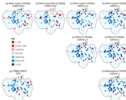
Figure 2.Full Kling–Gupta efficiency (KGE) scores at the 75 hydrological gauging stations for all simulations. For the periods 1997–2015 and 2004–2015 for the Coupled Routing and Excess Storage, Ensemble Framework for Flash Flood Forecasting (CREST EF5) run (g). Values greater than 0.75 are considered to indicate good performance (i.e. dark blue circles). To allow for easier model comparisons, plots are arranged by the different precipitation datasets (rows) and routing models (columns), with the exception of CREST EF5 (g). For example, the final column consists of model runs using the calibrated Lisflood routing model.

3.1 How well is the annual hydrological regime represented?

The annual hydrological regime on average is well repre-sented by all models (Fig. 2), with the rationale for poorer performance at specific gauges dependent on either the tem-poral correlation, bias ratio, or variability ratio components of the KGE (Figs. 3–5). An average of 50 % of stations note scores above 0.5 for the KGE metric across all eight simu-lated runs, with a maximum value of 0.92 observed at the Santa Rosa gauging site (48, Fig. 1a) for the ERA-5 Lis-flood_c simulation (Fig. 2f). The two CaMa-Flood set-ups using the PCR-GLOBWB hydrological model and the H-TESSEL LSM show the lowest skill, with 19 and 18 stations noting scores greater than 0.5 respectively. By contrast, the best performance is from the calibrated Lisflood set-ups, with median scores across stations of 0.56, 0.63, and 0.64 for runs forced with Interim Land, the reforecasts, and ERA-5 respectively. Such results are unsurprising given that the KGE was used as the objective function in the calibration algorithm of the Lisflood routing model.

In terms of spatial distribution, the poorest performance is consistent for the majority of simulations at the Arapari (55), Boca Do Inferno (56), and Base Alalau (61) gauging sta-tions located north of Manaus, at the Fazenda Cajupiranga gauge (64) in the northernmost Branco catchment, and at the Fontanilhas (35) and Indeco (49) stations in the south-eastern Brazilian Amazon (Fig. 2). In the south-south-eastern Ama-zon, particularly in the Madeira and Tapajos sub-basins, the number of existing or under-construction dams is at its high-est (Fig. 1b). Damming of rivers is known to have impacts on different aspects of the flow regime, with possible alter-ations in the timing, magnitude, and frequency of low and high flows (Magilligan and Nislow, 2005). Indeed, the fre-quency and duration of low- and high-flow pulses at stations downstream of dams have been shown to be particularly af-fected by the construction of cumulative dams (Timpe and Kaplan, 2017). Thus, discrepancies between observed and modelled data shown in Fig. 2 could be due to alterations to key features of the flow regime.

where the network of tributaries remains relatively unaf-fected by damming and where slopes are gentle (Fig. 1b and d). However, high skills at stations (32, 33, and 43) along the Madeira River for most simulations (Fig. 2) highlight that the impacts of hydroelectric dams need to be consid-ered on an individual basis, with two of the largest dams (>3000 MW) situated along the river (see Fig. 1b).

Figures 3–5 show the breakdown of the KGE scores for each hydrological component to evaluate differences in per-formance with respect to the correlation (i.e. timing), flow variability (α), and bias ratio (β). An average of 79 % of stations note correlation coefficients exceeding 0.6 across all runs, with those using the Lisflood routing model performing similarly in both spatial distribution and magnitude (Fig. 3). In contrast, 51 % and 47 % of stations achieve values ex-ceeding 0.6 for CaMa-Flood H-TESSEL and CaMa-Flood PCR-GLOBWB respectively, with the hydrological model, PCR-GLOBWB, noting better performance at stations along the main stem. The increased performances of Lisflood rela-tive to simulations incorporating CaMa-Flood are likely due to the increased spatial resolution of the routing component (see Table 1). This is supported by results for CREST EF5, with 76 % of stations noting values above 0.6 and the model occupying a finer spatial resolution than that of CaMa-Flood (Fig. 3g).

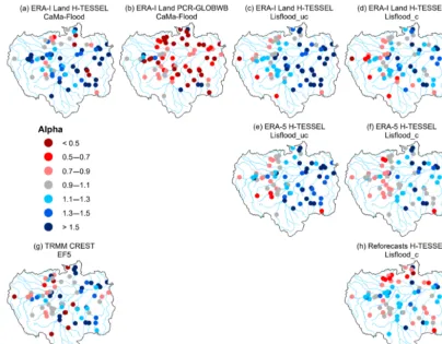
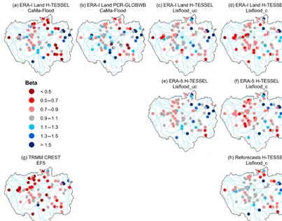
The variance of modelled river flow is on average higher than the observed time series in all of the simulations, with the exception of the ERA-Interim Land PCR-GLOBWB CaMa-Flood simulation. For this run, 85 % of stations ob-serve values of less than one, with stations situated in the Pe-ruvian Amazon (2–5) the notable exception (Fig. 4b). In con-trast, 79 % of stations for the CaMa-Flood set-up using the H-TESSEL LSM note values greater than one (Fig. 4a). All runs tend to underestimate river flows relative to the observed time series, with the majority of stations observing a beta value of less than one (Fig. 5). In the calibrated Lisflood simulation forced with the reforecasts, almost half of all the stations ob-serve scores between 0.9 and 1.1 (i.e. grey circles), with a median of 0.99 (Table 2). These results are not replicated in the other two calibrated runs when using either ERA-Interim Land or ERA-5 as the precipitation input (Fig. 5d and f). For both of these runs a decrease is found in the number of sta-tions achieving scores between 0.9 and 1.1 relative to the as-sociated uncalibrated Lisflood set-ups (Fig. 5c and e). This is also highlighted by a decrease in the median scores of the two respective runs (Table 2), meaning that a greater water deficit exists in the calibrated set-ups.

Stations in the south-eastern Amazon, particularly in the upper reaches of the Teles Pires River (37, 38, and 49), tend to underestimate river flow for most simulations (Fig. 5). In this region of the basin precipitation is controlled by frontal systems in the South Atlantic Convergence Zone (SACZ), which is prevalent during austral summer (Ronchail et al., 2002; Espinoza et al., 2009). In addition, rainfall variability in the Amazon is strongest in the south-east, with a distinct

dry season (Paiva et al., 2012; Espinoza et al., 2009). Further analysis could be useful in evaluating seasonal patterns of model performance to establish whether climatological fea-tures such as the SACZ are accurately represented within the precipitation datasets. Other factors impacting performance in the south-east could be associated with the geology and topography (Fig. 1c and d). Stations in this area of the basin are located within the Brazilian Shields, composed predom-inately of Precambrian rock, and are characterized by gen-tle slopes and low erosion rates (Filizola and Guyot, 2009). Paiva et al. (2012) demonstrated the importance of accu-rate initial conditions of groundwater state variables in the Tapajos and Xingu river basins, particularly for low flows. In comparison, the majority of the central parts of the basin are characterized by tertiary rocks, flat terrain, large flood-plains, and high sediment yields. In these regions (e.g. in the south-western Brazilian Amazon), KGE scores are generally higher (Fig. 2), with surface water variables (e.g. water lev-els, surface runoff, and floodplain storage) considered more important in hydrological prediction uncertainties (Paiva et al., 2012).

The KGE allows us to make explicit interpretations of the hydrological performance of each model owing to decom-position into correlation, bias, and variability terms (Kling et al., 2012). The results indicate that the required develop-ments to improve the representation of daily river flows are specific to each individual model and to the area of inter-est. For instance, for the ERA-Interim Land PCR-GLOBWB run, daily correlation scores (Fig. 3b) showed the model suf-fers in reproducing the temporal dynamics of flow (as mea-sured byr) in northern catchments. Calibration of parame-ters which control the timing of the flood wave (e.g. river flow velocity) may improve performance, whereas model set-ups incorporating the uncalibrated Lisflood routing model generally had lower KGE values in the east of the basin corresponding to an overestimation of river flow variabil-ity (Fig. 4c and e). For these runs, performance slightly im-proved upon the calibration of the groundwater and routing parameters relating to timing, flow variability, and ground-water loss (Fig. 4d and f).

3.2 Which model set-up best represents annual maximum river flows?

Figure 3.Correlation component (Pearson’s) of the KGE at the 75 hydrological gauging stations for all simulations. For the periods 1997– 2015 and 2004–2015 for the Coupled Routing and Excess Storage, Ensemble Framework for Flash Flood Forecasting (CREST EF5) run (g). Values greater than 0.6 are considered skilful (i.e. blue circles).

Table 2.Median scores for the 75 hydrological gauging stations for all metrics.

Model runs Spearman KGE r Beta Alpha

annual max (Pearson’s)

correlations

ERA-Interim Land H-TESSEL CaMa-Flood 0.24 0.30 0.61 0.92 1.33

ERA-Interim Land PCR-GLOBWB CaMa-Flood 0.23 0.18 0.59 0.98 0.64

ERA-Interim Land H-TESSEL Lisflood_uc 0.40 0.51 0.80 0.99 1.25

ERA-Interim Land H-TESSEL Lisflood_c 0.42 0.56 0.80 0.86 1.15

ERA-5 H-TESSEL Lisflood_uc 0.53 0.63 0.85 0.97 1.26

ERA-5 H-TESSEL Lisflood_c 0.54 0.64 0.86 0.87 1.06

TRMM CREST EF5 0.24 0.46 0.71 0.80 1.08

Reforecasts H-TESSEL Lisflood_c 0.32 0.63 0.83 0.96 1.06

Median across models 0.35 0.50 0.78 0.91 1.11

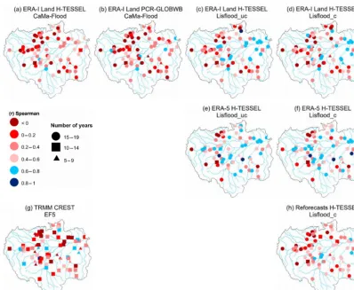
and therefore the spatial distribution of model performance should be interpreted with caution. To provide a certain level of confidence between results, stations whose time se-ries equals or exceeds 15 years are denoted using a circle, whereas those between 10–14 and 5–9 are represented using a square and triangle respectively.

The highest scores are generally located towards the east-ern side of the basin and along the main Amazon River where

Figure 4. Alpha (i.e. variability ratio) component of the KGE at the 75 hydrological gauging stations for all the simulations. For the periods 1997–2015 and 2004–2015 for the Coupled Routing and Excess Storage, Ensemble Framework for Flash Flood Forecasting (CREST EF5) run (g). Blue circles indicate that the variability in the simulated time series is higher than that of the observed one, while red circles show the opposite effect. Values closer to one indicate better model performance (i.e. grey circles).

mean precipitation totals over the validation period (1997– 2015), the reforecasts observe lower precipitation totals over central to northern areas of the basin relative to both of the climate reanalysis datasets (Fig. 8). However, when compar-ing the results of the ERA-Interim Land H-TESSEL CaMa-Flood and ERA-Interim Land H-TESSEL Lisflood_uc set-ups, correlations are much lower in the CaMa-Flood simula-tion, suggesting that both precipitation and routing processes are equally important (Fig. 6a and c).

Low agreement between peaks is consistent in the south-east and north-west of the basin across all simulations (Fig. 6). In the south-east, a lack of skill could again be asso-ciated with the abundance of hydroelectric dams in the region or with the poor representation of the SACZ rainfall regime. Evaluating the ability to represent the timing and magnitude of the annual flood wave has important implications for mod-els predicting flood hazard and for practices providing early warning information. These results identify that while the representation of daily river flows improves upon model cal-ibration of the Lisflood routing model (Sect. 3.1), the influ-ence of routing calibration for simulating flood peaks has no impact.

3.3 Which is the best-performing hydrological routing model?

We assessed the performance of the CaMa-Flood and Lis-flood_uc routing models by comparing the two runs which are forced using the ERA-Interim Land reanalysis dataset. On average the uncalibrated Lisflood run outperforms CaMa-Flood for all metrics analysed (Fig. 7 and Table 2). Results from the CREST EF5 model are also discussed but are not directly comparable due to using differing meteorological in-puts.

Figure 5.Beta (i.e. bias ratio) component of the KGE at the 75 hydrological gauging stations for all the simulations. For the periods 1997– 2015 and 2004–2015 for the Coupled Routing and Excess Storage, Ensemble Framework for Flash Flood Forecasting (CREST EF5) run (g). Blue circles indicate that the bias in the simulated time series is higher than that of the observed one, while red circles show the opposite effect. Values closer to one indicate better model performance (i.e. grey circles).

the CREST EF5 simulation fits between the CaMa-Flood and Lisflood runs with a median daily correlation score of 0.71 and notes 12 stations which have scores greater than 0.8 (Fig. 3g).

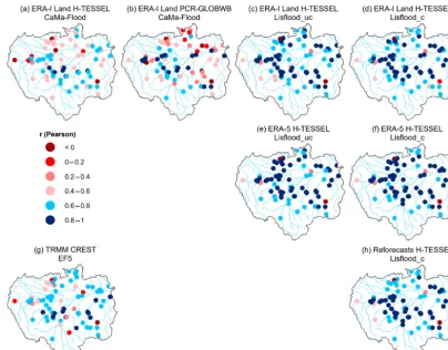
For the overall KGE metric, 24 % and 3 % of stations have values exceeding 0.5 and 0.75 for CaMa-Flood. These figures rise to 52 % and 11 % respectively in the uncali-brated Lisflood run. Large differences are particularly no-table at stations situated in the upper reaches of the Solimões River (2–6) and within a cluster of stations situated towards the Colombian Amazon in the north-west (Fig. 2c). Signifi-cant differences are identified for peak flow correlations, with only three stations (27, 17, and 22) achieving scores exceed-ing 0.6 for the CaMa-Flood simulation compared to 22 us-ing the uncalibrated Lisflood routus-ing scheme (Fig. 6a and c). In comparison, the CREST EF5 simulation has 11 stations exceeding this threshold, with no distinguishable spatial pat-tern (Fig. 6g). For this run, the time series of modelled data is shorter (2004–2015), and so peak flow correlations should be interpreted with caution.

Stations located in and around the main Amazon River ob-serve better performance for representing flood peaks in the

Lisflood simulation (Fig. 6c), aligning with the locations of lakes included within the Lisflood set-up (see Zajac et al., 2017). This level of skill was not replicated in the CaMa-Flood simulation, where the representation of lakes is not in-cluded (Fig. 6a), suggesting the potential importance of lake parameterization for accurate peak flow estimations. How-ever, Zajac et al. (2017) demonstrated that although the in-clusion of lakes in Lisflood was found to generally improve the representation of extreme discharge for the 5- and 20-year return periods on the global domain, the change in skill upon the inclusion of lakes and reservoirs in the Amazon was minimal for several metrics. Very few reservoirs are included within Lisflood in the Amazon, and therefore the estimated effects on simulated streamflow are restricted.

Figure 6.Spearman’s ranked correlation coefficients for observed against simulated annual maximum discharge values at the 75 hydrological gauging stations for all simulations. For the periods 1997–2015 and 2004–2015 for the Coupled Routing and Excess Storage, Ensemble Framework for Flash Flood Forecasting (CREST EF5) run (g). Values exceeding 0.6 are considered skilful (i.e. blue shapes). The number of overlapping years of data between observations and simulations are denoted by different shapes. A triangle represents 5–9 years, a square 10–14 years, and a circle 15–19 years of overlapping data.

is most suitable for certain applications within the Amazon basin. Results suggest that adjustments of certain parameters such as Manning’s channel coefficient could potentially im-prove the performance of the CaMa-Flood model, with the default coefficient higher in the uncalibrated Lisflood set-up (0.10 as opposed to 0.03; see Hirpa et al., 2018, for all default parameter values).

3.4 Which is the best-performing precipitation dataset? Three precipitation products (ERA-Interim Land, ERA-5, and the reforecasts) are used to force the calibrated Lisflood routing model, with the most recent ERA-5 reanalysis prod-uct the best-performing dataset. Figure 8 displays mean daily precipitation totals for each dataset over the main validation period (1997–2015). The main differences can be seen in the far west of the basin towards the Andes mountains, where precipitation is higher in ERA-5 compared to ERA-Interim Land, and in the north-west, where average daily precipita-tion totals are smaller in the reforecasts. On the other hand, values in the south-eastern corner of the basin are very

sim-ilar between the three datasets. When comparing observed and simulated annual peak flows, median correlation scores improve by 0.12 and 0.22 when using ERA-5 compared to when using ERA-Interim Land and the reforecasts respec-tively (Table 2); 28 stations reach the 0.6 threshold relative to 22 and 9 stations for ERA-Interim Land and the refore-casts respectively, with the range of coefficients smaller for ERA-5 (Fig. 7a).

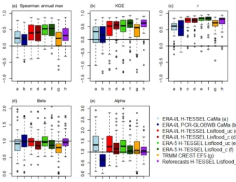
Figure 7.Boxplots showing the distribution of scores for the(a)Spearman annual maximum correlation,(b)KGE,(c)KGE Pearson’s

coefficient,(d)KGE beta, and(e)KGE alpha, for all simulations. For the period 1997–2015.

Figure 8.Mean daily precipitation totals throughout the Amazon basin. For(a)ERA-Interim Land,(b)ERA-5, and(c)the European Centre for Medium-Range Weather Forecasts (ECMWF) 20-year reforecasts. For the period 1997–2015.

In the other main tributary to the Solimões River, the Ucayali River, simulated annual peak flows show little agree-ment with observed data, with a decrease in skill identi-fied when using ERA-5 as opposed to ERA-Interim Land (Fig. 9e). Despite the lack of agreement between observed and modelled data in the Ucayali River, the higher correla-tion scores identified downstream at Tamshiyacu suggest that better representation of high-water periods at the start of the Solimões River is likely modulated by the larger Marañón River. Therefore, the ability to represent flood hazard in com-munities near to the city of Iquitos is more dependent on how well we can predict river flow in the Marañón River.

All three runs perform well for the KGE metric, with little difference in results spatially (Fig. 2d, f, h). The re-forecast simulation used within the Lisflood calibration is

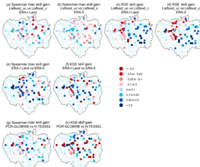
Figure 9.Relative improvement in skill at each gauging station for Spearman annual maximum correlations and KGE values (i.e. skill

scores).(a–d)show relative gain or loss in skill when using the calibrated Lisflood run (Lisflood_c) relative to the uncalibrated model run

(Lisflood_uc), using precipitation forcing from both ERA-Interim Land and ERA-5.(e)and(f)show the relative gain or loss in skill when

using ERA-5 as opposed to ERA-Interim Land.(g)and(h)show the relative gain or loss in skill when using the land surface model (LSM),

the Hydrology-Tiled ECMWF Scheme for Surface Exchanges over Land (H-TESSEL), compared to the hydrological model, PCRaster Global Water Balance (PCR-GLOBWB). All scores are calculated using the skill scores in Eq. (1). Red circles indicate a decrease in skill, whereas blue circles represent an increase.

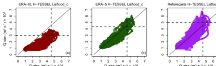
The Tamshiyacu gauging station (4) is used to measure flood hazard in the city of Iquitos at the start of the Solimões River (Espinoza et al., 2013) and is therefore of particu-lar interest. At this important location, scatterplots of ob-served against simulated river discharge (Fig. 10) show that the negative bias observed when using ERA-Interim Land is corrected for when using ERA-5, with the magnitude of the 90th percentile of river flows almost identical to that of the observed dataset. Improvement is likely associated with the increased resolution of the ERA-5 reanalysis, which ob-serves higher daily mean precipitation totals in regions to-wards the Andes in the far north-west of the basin (Fig. 8b). Waters found at Tamshiyacu are of Andean origin, meaning that the representation of rainfall in the Andes Mountains is fundamental to accurately predicting streamflow. ERA-5 runs at a horizontal resolution of ∼31 km and includes an additional 73 vertical levels to 0.01 hPa compared to

ERA-Interim Land, meaning the representation of the troposphere is enhanced (ECMWF, 2017).

fu-Figure 10. Scatterplots of observed against simulated river flow at the Tamshiyacu gauging site, Peru (4). For(a)ERA-Interim Land,

(b)ERA-5, and(c)the European Centre for Medium-Range Weather Forecasts (ECMWF), 20-year reforecasts forced through the calibrated

Lisflood routing model. Dashed black lines indicate the observed and simulated 90th percentile of river flow. For the period 1997–2015.

ture work, it could be of interest to compare the performance of ERA-5 against a wider range of precipitation datasets, such as the Multi-Source Weighted-Ensemble Precipitation (MSWEP) product that carefully integrates gauge, satellite, and reanalysis-based estimates. The Beck et al. (2017b) eval-uation of 22 precipitation datasets previously demonstrated the advantages of using merged products for hydrological modelling purposes.

3.5 How do results differ between using a LSM and a hydrological model?

The H-TESSEL LSM and the PCR-GLOBWB hydrological model are directly compared whereby the precipitation forc-ing (ERA-Interim Land) and river routforc-ing scheme (CaMa-Flood) are consistent. Overall, it appears that the choice be-tween using a LSM or a hydrological model in the Amazon basin is dependent not only on the specific region of interest, but also on the application and needs of the user. Previous studies (Zhang et al., 2016; Beck et al., 2017a) have found that LSMs, on average, perform better in rainfall-dominant regions, whereas hydrological models tend to achieve bet-ter results in snow-dominated regions owing to the use of complex energy balance equations introducing additional un-certainties. For the Amazon basin, Spearman’s rank correla-tion coefficients between simulated and observed peak river flow are closely matched, with medians of 0.24 and 0.23 for H-TESSEL and PCR-GLOBWB respectively (Table 2). However, the number of stations with Spearman’s maxi-mum correlation scores exceeding 0.6 is slightly higher in PCR-GLOBWB at seven compared to three with H-TESSEL (Fig. 6a and b).

To illustrate the gain or loss in skill when using H-TESSEL relative to PCR-GLOBWB, Spearman’s annual maximum correlation and KGE skill scores were calculated for each station (Fig. 9g and h). Overall, 68 % of the stations show improved skill for peak river flow correlations when using the LSM, though the gain in skill is minimal (median correlation skill score=0.06). This percentage drops to 37 % and 22 % for improvements in skill which exceed 0.1 and 0.2 respectively (Fig. 9g). By contrast, over half of the stations

see improvements in the KGE skill score for the hydrologi-cal model, PCR-GLOBWB, and 23 % of the stations observe KGE skill score increases which exceed 0.25 (Fig. 9h).

A large loss in performance for the KGE is observed when using H-TESSEL for stations in the Peruvian Amazon at the confluence point to the Solimões River (Fig. 9h). Model per-formance in this region can largely be attributed to the failure of the H-TESSEL CaMa-Flood run to accurately represent the variance of flow and the temporal correlation component of the KGE, with the variability of modelled flow far higher than in the observed data (Fig. 4a). Northern regions in the Branco basin and stations situated towards the Colombian Amazon show the opposite effect with higher KGE coeffi-cients found for the H-TESSEL CaMa-Flood run (Fig. 2a), indicating that model suitability is regionally specific. 3.6 By how much does the calibration of groundwater

Overall, hydrological performance improves upon model parameter calibration, with positive KGE skill scores (i.e. an increase in skill) at 61 % (59 %) of gauging stations for simulations forced with ERA-Interim Land (ERA-5) (Fig. 9c and d). The influence of calibration is stronger for the simula-tion forced with ERA-5, with the number of stasimula-tions achiev-ing “intermediate” KGE scores (i.e. 0.75>KGE_>0.5) to-talling 53 compared to 43 for ERA-Interim Land, an increase of 9 and 12 stations relative to the associated uncalibrated runs. When observing the spatial distribution of relative im-provements, an east–west divide can be seen (Fig. 9c and d). Generally, decreases in skill are concentrated to stations on the western side of the basin, whereas stations located to the east display improved hydrological representation.

Three stations (2–4) in the Peruvian Amazon show in-creased KGE skill scores when using the calibrated ERA-5 run relative to the similar uncalibrated set-up (Fig. 9d). Con-versely, a loss in skill is observed at each station for the cal-ibrated run forced using ERA-Interim Land (Fig. 9c). These results are likely associated with a larger negative runoff bias within the ERA-Interim Land Lisflood_uc run relative to the ERA-5 Lisflood_uc simulation for the three stations (Fig. 5c and e). This is supported by Hirpa et al. (2018), who con-cluded that stations which have a negative streamflow bias in the default run (i.e. Lisflood_uc) also have a negative KGE skill score in the calibrated simulation owing to the challenge of correcting for a water deficit within the routing compo-nent. Thus, for GHMs which tend to underestimate runoff, adjustments of parameters within the LSM or hydrological model (e.g. those responsible for the portioning of precipita-tion into runoff) or through bias-correcprecipita-tion measures within the precipitation dataset may be advantageous in efforts to accurately represent floods.

No significant differences between calibrated and uncali-brated Lisflood annual maximum correlation scores are iden-tified (Fig. 7a and Table 2). In total, the number of stations exceeding the 0.6 threshold for peak flow correlations re-mains the same for runs involving ERA-5 and decreases by one for ERA-Interim Land, meaning that the routing model calibration has very little impact on the ability to capture an-nual peaks. This suggests that calibrated parameters control-ling flow timing (e.g. Manning’s channel coefficient) are not as important for simulating the magnitude of higher flows in the Amazon basin and that bias correction of the precip-itation or calibration of parameters associated with runoff and evapotranspiration might be more useful. As previously highlighted by Hirpa et al. (2018), the inclusion of an ob-jective function that is explicitly based on flood peaks could improve the ability of Lisflood to simulate floods. This is supported by previous studies (Greuell et al., 2015; Beck et al., 2017a; Mizukami et al., 2019) which have also identi-fied that improved performance in calibrated models is pre-dominately specific to metrics which are incorporated into the objective function used within the calibration. For in-stance, in Mizukami et al. (2019), they find that when using

an application-specific metric (annual peak flow bias; APFB) for the calibration of two hydrological models, it produced the best peak flow annual estimates compared to using the NSE, KGE, and its components. However, despite this im-provement, flood magnitudes were still underestimated for all metrics used in calibration, and the use of the APFB as the calibration metric resulted in poorer performance across the individual KGE components upon evaluation.

3.7 Limitations and future work

While estimating the magnitude of peak river flows is funda-mental, more evaluation is required in assessing the ability to represent the timing of flood peaks. Modelled flood peaks have been known to occur too early in large Amazonian rivers (Alfieri et al., 2013; Hoch et al., 2017b), with accurate flow timing of significant importance in the Amazon basin. For example, the time displacements between peak flows in coinciding tributaries are known to play a major role in the dampening of the Amazon flood wave (Tomasella et al., 2010) and in the synchronization of flood peaks, commonly associated with exceptional flood events (e.g. Marengo et al., 2012; Espinoza et al., 2013; Ovando et al., 2016). Additional evaluation using metrics which focus specifically on the tim-ing aspect, such as the delay index (Paiva et al., 2013), would enable a more complete assessment of the hydrological mod-elling regime.

4 Conclusions

In this paper, eight different GHMs were employed in an in-tercomparison analysis using two verification metrics to as-sess model performance against gauged river discharge ob-servations. The motivation for this work stemmed from the need to evaluate the ability of GHMs to reproduce historical floods in the Amazon basin for use in climate analysis and to identify the strengths and weaknesses which exist along the hydrological modelling chain in order to provide insight to model developers. The implications of these results suggest that the choice of precipitation dataset is the most influen-tial component of the GHM set-up in terms of our ability to recreate annual maximum river flows in the Amazon basin. This is evident with average station correlations between ob-served and simulated annual maximum river flows increas-ing when usincreas-ing the new ERA-5 reanalysis dataset, with sig-nificant improvements in locations of the Peruvian Ama-zon. In this region, waters are sourced from Andean origins where rainfall can often be poorly represented due to topo-graphically complex terrains (Paiva et al., 2013). Thus, those wishing to simulate higher flows in the upper reaches of the Amazon may benefit from choosing a precipitation dataset which has a high spatial resolution, whereby the upper atmo-sphere is discretized at finer scales. Although an exact recom-mended spatial resolution cannot be provided based on the results of this study alone, previous works (e.g. Beck et al., 2017b) support the need for a comparatively high-resolution dataset in addition to other advantageous factors such as a long temporal record and the inclusion of daily gauge cor-rections.

Although parameter calibration of the Lisflood routing model improved the representation of the whole hydrologi-cal regime across the basin, the agreement between observed and simulated peak discharge values saw no change upon cal-ibration. This indicates that the benefit of calibration is con-fined to the objective function used, in this case the KGE, and highlights that further model calibration using an objective function that fits the purpose of the application (e.g. RMSE of flood peaks or APFB for flood forecasting systems) could be worth considering. It is important to reiterate however that thoughtful consideration is required if choosing application-specific metrics, with the potential to degrade performance in other aspects of the hydrological regime (e.g. bias and flow variability ratios) a concern (Mizukami et al., 2019). The rel-ative importance of good performance in the specific target metric compared to better performance for a range of metrics should be assessed on a model-by-model and circumstantial basis, taking into account the needs of potential users.

Data availability. All of the data and models used in this study were obtained from collaborators of the Global Flood Partner-ship (GFP) and are freely available. Access to these sources is men-tioned in Sect. 2.

Supplement. The supplement related to this article is available online at: https://doi.org/10.5194/hess-23-3057-2019-supplement.

Author contributions. EZ provided data and information for all simulations incorporating Lisflood and for the ERA-Interim Land H-TESSEL CaMa-Flood set-up. ZF and JM provided data and information for the TRMM CREST EF5 and ERA-Interim Land PCR-GLOBWB CaMa-Flood runs respectively. ES, HC, JB, and EC supervised the research and provided important advice. ES, HC, and JT designed the analysis and JT undertook the research in addition to writing the paper. All the authors were involved in discussions throughout the development and commented on the manuscript.

Competing interests. The authors declare that they have no conflict of interest.

Acknowledgements. Jamie Towner is grateful for financial sup-port from the Natural Environment Research Council (NERC) as part of the SCENARIO Doctoral Training Partnership (grant agree-ment NE/L002566/1). The first author is grateful for travel sup-port and funding provided by the Red Cross Red Crescent Climate Centre, to the research and national services, SO-HYBAM, IRD, SENAMHI, ANA, and INAMHI, for providing observed river dis-charge data, and to the ECMWF for computer access and techni-cal support. Finally, specific thanks go to Christel Prudhomme and the Environmental Forecasts team in the Evaluation Section at the ECMWF for their advice and support throughout the analysis and writing of the manuscript.

Financial support. This research has been supported by the SCE-NARIO NERC (grant no. NE/L002566/1).

Review statement. This paper was edited by Stacey Archfield and reviewed by Gemma Coxon and Andrew Newman.

References

Alfieri, L., Burek, P., Dutra, E., Krzeminski, B., Muraro, D., Thie-len, J., and Pappenberger, F.: GloFAS – global ensemble stream-flow forecasting and flood early warning, Hydrol. Earth Syst. Sci., 17, 1161–1175, https://doi.org/10.5194/hess-17-1161-2013, 2013.

Alfieri, L., Cohen, S., Galantowicz, J., Schumann, G. J., Trigg, M. A., Zsoter, E., Prudhomme, C., Kruczkiewicz, A., Cough-lan de Perez, E., Flamig, Z., Rudari., R., Wu, H., Adler, R. F., Brakenbridge, R. G., Kettner, A., Weerts, A., Matgen, P., Is-lam, S. A. K. M., and Salamon, P.: A global network for oper-ational flood risk reduction, Environ. Sci. Policy, 84, 149–158, https://doi.org/10.1016/j.envsci.2018.03.014, 2018.

atmo-spheric reanalysis datasets be used to reproduce flooding over large scales?, Geophys. Res. Lett., 44, 10369–10377, https://doi.org/10.1002/2017GL075502, 2017.

Andreadis, K. M., Schumann, G. J. P., Stampoulis, D., Bates, P. D., Brakenridge, G. R., and Kettner, A. J.: Can Atmo-spheric Reanalysis Data Sets Be Used to Reproduce Flood-ing Over Large Scales?, Geophys. Res. Lett., 44, 10369–10377, https://doi.org/10.1002/2017GL075502, 2017.

Arnell, N. W. and Gosling, S. N.: The impacts of climate change on river flood risk at the global scale, Climatic Change, 134, 387– 401, https://doi.org/10.1007/s10584-014-1084-5, 2016. Balsamo, G., Beljaars, A., Scipal, K., Viterbo, P., van den Hurk,

B., Hirschi, M., and Betts, A. K.: A revised hydrology for the ECMWF model: Verification from field site to terrestrial water storage and impact in the Integrated Forecast System, J. Hydrom-eteorol., 10, 623–643, https://doi.org/10.1175/2008JHM1068.1, 2009.

Balsamo, G., Pappenberger, F., Dutra, E., Viterbo, P., and Van den Hurk, B. J. J. M.: A revised land hydrology in the ECMWF model: a step towards daily water flux prediction in a fully-closed water cycle, Hydrol. Process., 25, 1046–1054, https://doi.org/10.1002/hyp.7808, 2010.

Balsamo, G., Albergel, C., Beljaars, A., Boussetta, S., Brun, E., Cloke, H., Dee, H., Dutra, D., Muñoz-Sabater, J., Pappen-berger, F., de Rosnay, P., Stockdale. T., and Vitart, F.: ERA-Interim/Land: a global land surface reanalysis data set, Hydrol. Earth Syst. Sci., 19, 389–407, https://doi.org/10.5194/hess-19-389-2015, 2015.

Balsamo, G., Agusti-Panareda, A., Albergel, C., Arduini, G., Bel-jaars, A., Bidlot, J., Bousserez, N., Boussetta, S., Brown, A., Buizza, R., Buontempo, C., Chevallier, F., Choulga, M., Cloke, H., Cronin, M. F., Dahoui, M., De Rosnay, P., Dirmeyer, P. A., Drusch, M., Dutra, E., Ek, M. B., Gentine, P., Hewitt, H., Keeley, S. P. E., Kerr, Y., Kumar, S., Lupu, C., Mahfouf, J. F., McNorton, J., Mecklenburg, S., Mogensen, K., Muñoz-Sabater, J., Orth, R., Rabier, F., Reichle, R., Ruston, B, Pap-penberger, F., Sandu, I., Seneviratne, S. I., Tietsche, S., Trigo, I. F., Uijlenhoet, R., Wedi, N., Woolway, R. L., and Zeng, X.: Satellite and In Situ Observations for Advancing Global Earth Surface Modelling: A Review, Remote Sens., 10, 2038, https://doi.org/10.3390/rs10122038, 2018.

Beck, H. E., van Dijk, A. I., de Roo, A., Dutra, E., Fink, G., Orth, R., and Schellekens, J.: Global evaluation of runoff from ten state-of-the-art hydrological models, Hydrol. Earth Syst. Sci., 21, 2881– 2903, https://doi.org/10.5194/hess-21-2881-2017, 2017a. Beck, H. E., Vergopolan, N., Pan, M., Levizzani, V., van Dijk, A. I.,

Weedon, G. P., Brocca, L., Pappenberger, F., Huffman, G. J., and Wood, E. F.: Global-scale evaluation of 22 precipitation datasets using gauge observations and hydrological modeling, Hydrol. Earth Syst. Sci., 21, 6201–6217, https://doi.org/10.5194/hess-21-6201-2017, 2017b.

Bergström, S.: The HBV model, in: Comput. Model. Watershed Hy-drol., chap. The HBV mo, edited by: Singh, V., Water Resouces Publications, Highlands Ranch Co., Colorado, USA, 1995. Beven, K. J.: Rainfall-Runoff Modelling: The Primer, 2nd Edn.,

Wiley-Blackwell, Chichester, UK, 2012.

Bierkens, M. F.: Global hydrology 2015: State, trends,

and directions, Water Resour. Res., 51, 4923–4947,

https://doi.org/10.1002/2015WR017173, 2015.

Bierkens, M. F., Bell, V. A., Burek, P., Chaney, N., Condon, L. E., David, C. H., de Roo, A., Döll, P., Drost, N., Famigiletti, J. S., Flörke, M., Gochis, D. J., Houser, P., Hut, R., Keune, J., Kollet, S., Maxwell, R. M., Reager, J. T., Samaniego, L., Sudicky, E., Sutanudiaia, E. H., van de Giesen, N., Winsemius, H., and Wood, E. F.: Hyper-resolution global hydrological modelling: what is next? “Everywhere and locally relevant”, Hydrol. Process., 29, 310–320, https://doi.org/10.1002/hyp.10391, 2015.

Bondeau, A., Smith, P. C., Zaehle, S., Schaphoff, S., Lucht, W., Cramer, W., Gerten, D., Lotze-Campen, H., Muller, C., Re-ichstein, M., and Smith, B.: Modelling the role of agriculture for the 20th century global terrestrial carbon balance, Global Change Biol., 13, 679–706, https://doi.org/10.1111/j.1365-2486.2006.01305.x, 2007.

Butts, M. B., Payne, J. T., Kristensen, M., and Madsen, H.: An eval-uation of the impact of model structure on hydrological mod-elling uncertainty for streamflow simulation, J. Hydrol., 298, 242–266, https://doi.org/10.1016/j.jhydrol.2004.03.042, 2004. Clark III, R. A., Flamig, Z. L., Vergara, H., Hong, Y.,

Gour-ley, J. J., Mandl, D. J., Frye, S., Handy, M., and Patterson, M.: Hydrological modeling and capacity building in the Re-public of Namibia, B. Am. Meteorol. Soc., 98, 1697–1715, https://doi.org/10.1175/BAMS-D-15-00130.1, 2016.

Correa, S. W., de Paiva, R. C. D., Espinoza, J. C., and Col-lischonn, W.: Multi-decadal Hydrological Retrospective: Case study of Amazon floods and droughts, J. Hydrol., 549, 667–684, https://doi.org/10.1016/j.jhydrol.2017.04.019, 2017.

Dee, D. P., Uppala, S. M., Simmons, A. J., Berrisford, P., Poli, P., Kobayashi, S., Andrae, U., Balmaseda, M. A., Balsamo, G., Bauer, P., Bechtold, P., Belijaars, A. C. M., van de Berg, L., Bid-lot, J., Bormann, N., Delsol, C., Dragani, R., Fuentes, M., Geer, A. J., Haimberger, L., Healy, S. B., Hersbach, S., Hólm, E .V., Isaksen, L., Kallberg, P., Köhler, M., Matricardi, M., McNally, A. P., Mong-Sanz, B. M., Morcrette, J. J., Park, B. K., Peubey, C., de Rosnay, P., Tavolato, C., Thèpaut, J. N., and Vitart, F.: The ERA-Interim reanalysis: Configuration and performance of the data assimilation system, Q. J. Roy. Meteorol. Soc., 137, 553– 597, https://doi.org/10.1002/qj.828, 2011.

De Groeve, T., Thielen-del Pozo, J., Brakenridge, R., Adler, R., Alfieri, L., Kull, D., Lindsay, F., Imperiali, O., Pappenberger, F., Rudari, R., Salamon, P., Villars, N., and Wyjad, K.: Join-ing forces in a global flood partnership, B. Am. Meteorol. Soc., 96, ES97–ES100, https://doi.org/10.1175/BAMS-D-14-00147.1, 2015.

Devia, G. K., Ganasri, B. P., and Dwarakish, G. S.: A re-view on hydrological models, Aquat. Proced., 4, 1001–1007, https://doi.org/10.1016/j.aqpro.2015.02.126, 2015.

Döll, P., Kaspar, F., and Lehner, B.: A global hydrological model for deriving water availability indicators: model tuning and vali-dation, J. Hydrol., 270, 105–134, https://doi.org/10.1016/S0022-1694(02)00283-4, 2003.

ECMWF: A brief description of reforecasts, available at: https://confluence.ecmwf.int/display/S2S/A+brief+description+ of+reforecasts (last access: 25 September 2018), 2016.

ECMWF: What are the changes from ERA-Interim to ERA5?,

available at: https://confluence.ecmwf.int//pages/viewpage.

action?pageId=74764925, (last access: 31 August 2018), 2017. ECMWF: What is ERA-5?, available at: https://confluence.ecmwf.