CAUSAL INFERENCE IN HIV/AIDS RESEARCH:
GENERALIZABILITY AND APPLICATIONS
Ashley L. Buchanan
A dissertation submitted to the faculty at the University of North Carolina at Chapel Hill in partial fulfillment of the requirements for the degree of Doctor of Public Health
in the Department of Biostatistics.
Chapel Hill 2014 Approved by: Michael G. Hudgens Adaora A. Adimora Shrikant I. Bangdiwala Stephen R. Cole Paul W. Stewart
c 2014 Ashley L. Buchanan ALL RIGHTS RESERVED
ABSTRACT
ASHLEY L. BUCHANAN: Causal Inference in HIV/AIDS Research: Generalizability and Applications
(Under the direction of Michael G. Hudgens)
In this research, we develop and apply causal inference methods for the field of infectious diseases. In the first part of this research, we consider an inverse probability (IP) weighted Cox model to estimate the effect of a baseline exposure on a time-to-event outcome. IP weighting can be used to adjust for multiple measured confounders of a baseline exposure in order to estimate marginal effects, which compare the distribution of outcomes when the entire population is exposed versus the entire population is unexposed. IP weights can also be employed to adjust for selection bias due to loss to follow-up. This approach is illustrated using an example that estimates the effect of injection drug use on time until AIDS or death among HIV-infected women.
In the second part of this research, we develop and apply methods for generalizing trial results for continuous data. In a randomized trial, assuming participants are a random sample from the target population may be dubious. Lack of generalizability can arise when the distribution of treatment effect modifiers in trial participants is different from the distribution in the target. We consider an inverse probability of sampling weighted (IPSW) estimator for generalizing trial results to a user-specified target population. The IPSW estimator is shown to be consistent and asymptotically normal. Expressions for the asymptotic variance and a consistent sandwich-type estimator of the variance are derived. Simulation results comparing the IPSW estimator to a previously proposed stratified estimator are provided. The IPSW estimator is employed to generalize results from the AIDS Clinical Trials Group (ACTG) to all people currently living with HIV in the U.S.
results for right-censored data. The IPSW estimator is considered for right-censored data and is defined as an inverse weighted Kaplan-Meier (KM) estimator. Simulation results are provided to compare this estimator to an unweighted KM estimator and a stratified estimator. The average standard error is computed using a nonparametric bootstrap. The IPSW estimator is employed to generalize survival results from the ACTG to all people currently living with HIV in the U.S.
To my parents, who were always supportive, and my dog, Jolie, who was always by my side.
ACKNOWLEDGMENTS
Many thanks to my committee members Dr. Adaora Adimora, Dr. Shrikant Bangdiwala, and Dr. Paul Stewart for their helpful comments. I would like to thank Dr. Michael Hudgens for guidance and inspiration that greatly strengthened this research. I would also like to thank Dr. Stephen Cole for providing me with the opportunity to apply causal inference methods and invaluable instruction on epidemiological research. I would also like to thank my friends in the Biostatistics and Epidemiology Departments, who made classes and research a joy: Amy Richardson, Tara Rao, Eric Jay Daza, Joe Rigdon, Catherine Lesko, and Katie Mollan. These findings are presented on behalf of the Women’s Interagency HIV Study (WIHS), the Center for AIDS Research (CFAR) Network of Integrated Clinical Trials (CNICS), and the AIDS Clinical Trials Group (ACTG). We would like to thank all of the WIHS, CNICS, and ACTG investigators, data management teams, and participants who contributed to this project. Funding for this study was provided by National Institutes of Health (NIH) grants R01AI100654, R01AI085073, U01AI042590, U01AI069918, R56AI102622, 5 K24HD059358-04, 5 U01AI103390-02 (WIHS), R24AI067039 (CNICS), and P30AI50410 (CFAR). The views and opinions expressed in this research do not necessarily state or reflect those of the NIH.
TABLE OF CONTENTS
LIST OF TABLES . . . ix
LIST OF FIGURES . . . xi
1 INTRODUCTION . . . 1
2 LITERATURE REVIEW . . . 3
2.1 Classical Causal Inference . . . 3
2.2 Inverse Probability Weighted Cox Models . . . 5
2.3 Generalizability of Randomized Trials . . . 8
2.3.1 Definitions and Background . . . 9
2.3.2 Sampling Score Methods to Generalize Trial Results . . . 12
2.3.3 Other Methods to Generalize Trial Results . . . 15
2.4 Methods for Generalizing Right-Censored Data . . . 17
2.5 Summary . . . 18
3 WORTH THE WEIGHT: USING INVERSE PROBABILITY WEIGHTED COX MODELS IN AIDS RESEARCH . . 20
3.1 Introduction . . . 20
3.2 Motivating Example: AIDS-Free Survival Among Injection Drug Users . . . . 21
3.3 Inverse Probability Weighted Cox Models . . . 22
3.4 Illustrative Example . . . 24
3.5 Discussion . . . 26
4 GENERALIZING EVIDENCE FROM RANDOMZIED TRIALS USING INVERSE PROBABILITY OF SAMPLING WEIGHTS . . . 38
4.2 Notation and Assumptions . . . 39
4.3 Estimators of the Population Average Treatment Effect . . . 41
4.4 Large Sample Properties of the Inverse Probability of Sampling Weighted Estimator . . . 42 4.5 Simulations . . . 45 4.6 Applications . . . 48 4.6.1 ACTG 320 . . . 48 4.6.2 ACTG A5202 . . . 51 4.7 Discussion . . . 54
5 GENEARLIZING TRIAL RESULTS FOR RIGHT-CENSORED DATA USING INVERSE PROBABILITY OF SAMPLING WEIGHTS . 67 5.1 Introduction . . . 67
5.2 Assumptions and Notation . . . 68
5.3 Estimators of the Marginal Survival Functions in the Target Population . . . 69
5.4 Simulations . . . 71 5.5 Applications . . . 73 5.5.1 ACTG 320 . . . 73 5.5.2 ACTG A5202 . . . 76 5.6 Discussion . . . 79 6 CONCLUSION . . . 98
Appendix A: Review of the Standard (Unweighted) Cox Pro-portional Hazards Model . . . 99
Appendix B: Sandwich Estimator of the Variance of the IPSW Estimator . 101 BIBLIOGRAPHY . . . 102
LIST OF TABLES
3.1 Characteristics of women in the Women’s Interagency HIV Study . . . 32 3.2 Association of history of injection drug use with time to AIDS
or death for women in the Women’s Interagency HIV Study . . . 33 3.3 Example individual-level estimated weights for women in the
Women’s Interagency HIV Study . . . 34
4.1 Summary of Monte Carlo results for estimators of the popula-tion average treatment effect when the sampling score model was
correctly specified . . . 57 4.2 Summary of Monte Carlo results for estimators of the population
average treatment effect when the sampling score model was misspecified . . 57 4.3 Characteristics of women in the Women’s Interagency HIV Study
and women in AIDS Clinical Trials Group 320 . . . 58 4.4 Difference in the average change in CD4 from baseline to week 4
between treatment groups for each level of the covariates among
women in AIDS Clinical Trials Group 320 . . . 58 4.5 Characteristics of participants in the CFAR Network of
Inte-grated Clinical Systems and participants in AIDS Clinical Trials
Group 320 . . . 59 4.6 Difference in the average change in CD4 from baseline to week 4
between treatment groups for each level of the covariates among
all participants in AIDS Clinical Trials Group 320 . . . 60 4.7 Characteristics of women in the Women’s Interagency HIV Study
and women in AIDS Clinical Trials Group A5202 . . . 61 4.8 Difference in the average change in CD4 from baseline to week 48
between treatment groups for each level of the covariates among
women in AIDS Clinical Trials Group A5202 . . . 62 4.9 Characteristics of participants in the CFAR Network of
Inte-grated Clinical Systems and participants in AIDS Clinical Trials
Group A5202 . . . 63 4.10 Difference in the average change in CD4 from baseline to week 48
between treatment groups for each level of the covariates among
4.11 Results for continuous outcomes in two AIDS Clinical Trials
Group trials . . . 65
5.1 Summary of Monte Carlo results among the treated for inverse probability of sampling weighted, stratified, and Kaplan-Meier
estimators of the marginal survival curves in the target population . . . 82 5.2 Summary of Monte Carlo results among the control for inverse
probability of sampling weighted, stratified, and Kaplan-Meier
estimators of the marginal survival curves in the target population . . . 83 5.3 Characteristics of women in the Women’s Interagency HIV Study
and women in AIDS Clinical Trials Group 320 . . . 84 5.4 Estimated risk difference at one year between treatment groups
for each level of the covariates among women in AIDS Clinical
Trials Group 320 . . . 85 5.5 Characteristics of participants in the CFAR Network of
Inte-grated Clinical Systems and participants in AIDS Clinical Trials
Group 320 . . . 86 5.6 Estimated risk difference at one year between treatment groups
for each level of the covariates among all participants in AIDS
Clinical Trials Group 320 . . . 87 5.7 Characteristics of women in the Women’s Interagency HIV Study
and women in AIDS Clinical Trials Group A5202 . . . 88 5.8 Estimated risk difference at week 48 between treatment groups
for each level of the covariates among women in AIDS Clinical
Trials Group A5202 . . . 89 5.9 Characteristics of participants in the CFAR Network of
Inte-grated Clinical Systems and participants in AIDS Clinical Trials
Group A5202 . . . 90 5.10 Estimated risk difference at week 48 between treatment groups
for each level of the covariates among participants in AIDS
Clin-ical Trials Group A5202 . . . 91 5.11 Results for the risk difference of the time-to-event outcomes in
two AIDS Clinical Trials Group studies . . . 92 5.12 Results for the risk ratio of the time-to-event outcomes in two
LIST OF FIGURES
3.1 Kaplan-Meier estimated AIDS-free survival curves for women in
the Women’s Interagency HIV Study . . . 35 3.2 Estimated log cumulative hazard curves without accounting for
any covariates for women in the Women’s Interagency HIV Study . . . 36 3.3 Standardized estimates of the log cumulative hazard curves for
women in the Women’s Interagency HIV Study . . . 37 4.1 Comparison of the distributions of intention-to-treat estimator,
inverse probability of sampling weighted estimator, and stratified
estimator based on 5,000 simulated datasets . . . 66 5.1 Simulation results for estimators of the marginal survival curves
with a right-censored outcome and a binary covariate . . . 93 5.2 Simulation results for estimators of the marginal survival curves
with a right-censored outcome and a continuous covariate . . . 94 5.3 Complement of the Kaplan-Meier survival curves among women
by treatment group in AIDS Clinical Trial Group 320 Study us-ing intent-to-treat and samplus-ing score weighted estimators. Rep-resentative cohort based on data from the Women’s Interagency
HIV Study. . . 95 5.4 Complement of the Kaplan-Meier survival curves by treatment
group in AIDS Clinical Trial Group 320 Study using intent-to-treat and sampling score weighted estimators. Representative cohort based on data from the CFAR Network of Integrated
Clinical Systems. . . 95 5.5 Complement of the Kaplan-Meier survival curves among women
by treatment group in AIDS Clinical Trial Group A5202 Study using intent-to-treat and sampling score weighted estimators. Representative cohort based on data from the Women’s
Inter-agency HIV Study. . . 96 5.6 Complement of the Kaplan-Meier survival curves by treatment
group in AIDS Clinical Trial Group A5202 Study using intent-to-treat and sampling score weighted estimators. Representative cohort based on data from the CFAR Network of Integrated
CHAPTER 1: INTRODUCTION
In this research, we develop and apply causal inference methods for the field of infectious diseases. In the first part of this research, we consider inverse probability (IP) weighted Cox models as an alternative to the standard Cox model. Survival analysis can be used in infectious disease research to compare the time to occurrence of clinical events between treatment or exposure groups (Cole and Hudgens, 2010). Randomized trials are the gold standard to estimate exposure effects on survival time, but are not always ethical or feasible. Although observational studies may provide estimates of effects when trial data are unavailable, the estimates they yield are often riddled with confounding (Greenland and Morgenstern, 2001). Informally, confounding occurs when the exposure and outcome share a common cause. The Cox proportional hazards regression model (Cox, 1972), the standard approach in survival analysis, can account for multiple measured confounders. As an alternative to the standard Cox model, we present a method in Chapter 3 that uses IP weights to estimate the effect of a baseline exposure on survival time. Under certain assumptions, results from an IP-weighted Cox model of observational data can be interpreted similar to a randomized trial with no drop out (i.e., loss to follow-up).
In the second part of this research, we develop and apply methods for generalizing trial results for continuous data. Results obtained in randomized trials may not generalize to a target population. Ideally, trial participants are a random sample from a target population and the treatment assignment mechanism is known to the analyst. In a randomized trial, the treatment assignment mechanism is always known, but trial participants are often a non-random sample from a target population. Lack of generalizability can arise when the distribution of treatment effect modifiers in trial participants is different from the distribution in a target population. Following Cole and Stuart (2010) and Stuart et al. (2011), we consider
an inverse probability of sampling weighted (IPSW) estimator for generalizing trial results to a target population. In Chapter 4, the IPSW estimator is shown to be consistent and asymptotically normal. Expressions for the asymptotic variance and a consistent sandwich-type estimator of the variance are also derived.
In the third part of this research, we develop and apply methods for generalizing trial results for censored data. In Chapter 5, the IPSW estimator is considered for right-censored data and is defined as an inverse weighted Kaplan-Meier (KM) estimator. Simulation results are provided to compare this estimator to an unweighted KM estimator and a stratified estimator. The average standard error is computed using a nonparametric bootstrap and performance is evaluated empirically. The IPSW estimator is employed to generalize survival results from the acquired immunodeficiency syndrome (AIDS) Clinical Trials Group (ACTG) to all people currently living with human immunodeficiency virus (HIV) in the U.S.
CHAPTER 2: LITERATURE REVIEW
2.1 Classical Causal Inference
Public health researchers are often interested in estimating causal effects of treatment or exposures using data from randomized clinical trials (RCTs) or observational studies. Causal inference is a paradigm to estimate effects and is often framed using potential outcomes (Little and Rubin, 2000). A potential outcome is defined as the outcome that would have been observed had a participant (possibly contrary to fact) been exposed to a certain level of treatment or exposure. In general, Yx is potential outcome under treatment X = 1 or lack of treatment X = 0. These potential outcomes are also referred to as factuals and counterfactuals in the literature (Morgan and Winship, 2007). This framework allows for ex-tensions beyond the randomized trial to accommodate scenarios such as observational studies, noncompliance, or missing data (Holland, 1986; Robins and Finkelstein, 2000; Rubin, 1990). The notation of potential outcomes is historically related to Neyman’s randomization-based inference (Neyman et al., 1992; Rubin, 1990; Robins, 1989). Once a participant is assigned to treatment, only one of the two potential outcomes is observed; thus, the problem of causal inference is akin to a missing data problem.
There are two randomization-based approaches to causal inference developed by Fisher (Fisher, 1973; Rubin, 1980) and Neyman et al. (1992). Using the Fisher approach, the sharp null hypothesis is evaluated, which states that the outcome is the same for both treatment groups for all participants (i.e., Yi1 = Yi0), where i indexes the study participants. Under the sharp null hypothesis, all information can be identified from the observed data (i.e., Y1
i = Yi0 = Yi) and test statistics and P values can be computed. Little and Rubin (2000) argued that this approach is limited because the null hypothesis is restrictive and significant tests may not be clinically meaningful.
In Neyman’s approach to causal inference, expectations of statistics are evaluated with respect to the distribution of the assignment mechanism and confidence intervals are calcu-lated for the average causal effect (Little and Rubin, 2000). This idea is historically recalcu-lated to Neyman’s randomization-based inference in surveys (Neyman et al., 1992). An unbiased estimator of the causal estimand and an unbiased (or upwardly biased) estimator of the vari-ance is derived. The central limit theorem allows for the construction of confidence intervals. Let ¯Y1 and ¯Y0 be the averages of the potential outcomes in the population. Let ¯y1 and ¯y0 denote the sample means among those assigned to treatment and control, respectively. Let n1 denote the number assigned to treatment, n0 denote the number assigned to control, s21 denote the variance among those assigned to treatment, and s20 denote the variance among those assigned to control. The estimated variance is se2 = s21/n1+ s20/n0. The 95% confidence interval for the average treatment difference ( ¯Y1− ¯Y0) is (¯y1− ¯y0) ± 1.96 × se. Neyman’s approach to causal inference is commonly used in epidemiological studies and is employed throughout this research.
There are several assumptions necessary to estimate causal effects. First, there needs to be no interference between participants and treatment variation irrelevance needs to hold (i.e., stable unit treatment value assumption (SUTVA)) (Rubin, 1980). This means that the potential outcomes for any participant do not vary with the treatments assigned to other par-ticipants, and, for each participant, there are no different forms or versions of treatment which lead to different potential outcomes. This implies that the study design needs a well-defined treatment assignment mechanism (Robins et al., 2000), so there are not multiple versions of exposure, or if there are, they are unimportant (Cole and Frangakis, 2009; Pearl, 2010; VanderWeele, 2009a). In general, consistency always holds (i.e., Y = Y1X + Y0(1 − X)). We must have measured enough variables so that we can effectively address confounding (Robins et al., 2000). Effectively addressing confounding can lead to exchangeability, which means the potential outcomes are independent of the exposure. In other words, the exposure assignment mechanism depends only on the data through the measured covariates and outcome (Little and Rubin, 2000). Confounders are variables associated with the exposure and independent risk factors for the outcome that are not affected by exposure (Greenland and Morgenstern,
2001). Informally, confounding occurs when exposure and outcome share a common cause. In a trial, exchangeability is gained through randomization. Lastly, the conditional proba-bility of receiving every level of treatment given covariates must be greater than zero (i.e., positivity) (Cole and Hernan, 2008).
Randomization of exposure allows for straightforward estimation of causal effects. In a completely randomized design, exposure is not associated with any potential confounders. Estimation of causal effects is not possible when there is unmeasured confounding. In many public health studies, it is not ethical or feasible to randomize the treatment or exposure. Principles of causal inference can be applied to estimate effects in observational studies in the presence of (measured) confounding. In section 2.2, we present the literature for IP-weighted Cox models, which is one approach to applying causal inference methods to estimate effects with observational data.
Causal inference methods can also be employed to sharpen inference from randomized trials. Informative censoring and generalizability of results are two possible concerns in trials (Cole and Stuart, 2010; Stuart et al., 2011; Frangakis and Rubin, 1999). A recent paper by Hernan et al. (2013) discussed how randomized trials may be subject to post-randomization selection bias and confounding, particularly for studies with longer follow-up. The authors argued that intention-to-treat analyses may not always be estimating the effects of inter-est. The authors also proposed a set of g-methods, including inverse probability weighting methods. In Section 2.3, we present the literature for generalizing trial results, highlighting recently proposed methods using sampling scores.
2.2 Inverse Probability Weighted Cox Models
The Cox proportional hazards regression model (Cox, 1972) is the standard approach to account for multiple measured confounders in observational studies with separate curves presented for each baseline covariate group. As an alternative to the standard Cox model, IP weights can be utilized to estimate the effect of an exposure that is fixed at study entry (Cole and Hernan, 2004; Nieto and Coresh, 1996; Xie and Liu, 2005). IP weighting creates a
pseudo-population in which confounders are no longer associated with the exposure. Under certain assumptions, results from an IP-weighted Cox model of observational data can be interpreted similar to results from a randomized trial with no drop out (i.e., loss to follow-up). One curve represents the survival if everyone (possibly contrary to fact) had been exposed at baseline, while the other curve represents the survival if no one (possibly contrary to fact) had been exposed at baseline (Cole and Hernan, 2004; Xie and Liu, 2005). Herein, we refer to IP weighting as standardization, where the standardization is to the entire population under two different exposures (Cole and Hernan, 2004; Sato and Matsuyama, 2003).
An IP-weighted Cox model is fit by maximizing a weighted partial likelihood accounting for confounding and possibly informative drop out measured by covariates through the estimated IP weight ˆwi(t). The estimated IP weight ˆwi(t) is the product of an estimated time-fixed IP exposure weight ˆw1i(t) and an estimated time-varying IP drop out weight ˆw2i(t) for each participant i at each survival time t. If certain assumptions are met, IP weighting can account for confounding and selection bias due to drop out by multiple covariates using both exposure and drop out weights. Standardized survival curve estimates can be obtained by fitting an IP-weighted Cox model stratified by exposure with no covariates and then nonparametrically estimating the baseline survival functions for the two strata, which are (asymptotically) equivalent to Kaplan-Meier estimates in the absence of weighting (Cole and Hernan, 2004; Collett, 2003).
The standardized (i.e., IP weighted) method provides potential benefits that the covariate-adjusted method lacks. First, results from the standardized approach can be used to mimic a randomized trial when only observational data is available (under certain assumptions). In particular, the estimated hazard ratio using the standardized approach can be interpreted the same as the (marginal) hazard ratio one would obtain in a randomized experiment such as a clinical trial where there is no drop out. In contrast, a covariate-adjusted Cox model hazard ratio does not necessarily equal the marginal hazard ratio (even in the absence of confounding) because the Cox model is not collapsible for the hazard ratio parameter (Greenland, 1996). A regression model is said to be collapsible for a parameter (in this case, the hazard ratio) if
the covariate-adjusted parameter is the same as the unadjusted parameter (Greenland et al., 1999b).
Second, the IP weighting approach yields standardized survival curve estimates. Although the hazard ratio is a common summary parameter to compare survival distributions between exposure groups, there are drawbacks to focusing inference on hazard ratios. For instance, the hazard ratio can be difficult to interpret, especially when trying to summarize the effect of a treatment or exposure (Hernan, 2010). Presenting estimated survival curves is an alternative to reporting hazard ratios that may be more interpretable because survival curves summarize all information from baseline up to any time t. The IP-weighted approach leads to Kaplan-Meier type survival curve estimates that are standardized to the entire population under two different exposures at baseline while accounting for confounding by multiple covariates. A covariate-adjusted Cox model does not afford such survival curve estimates (Cole and Hernan, 2004; Xie and Liu, 2005).
Third, the IP-weighted approach with drop out weights requires a weaker assumption about censoring than the covariate-adjusted Cox model. Specifically, if there are measured time-varying covariates predictive of censoring and survival time, the IP-weighted approach will yield consistent estimates of the marginal hazard ratio, while the covariate-adjusted Cox model estimator will not be consistent for the marginal or conditional hazard ratio (Hernan et al., 2000; Robins et al., 2000; Robins and Finkelstein, 2000).
When interest focuses on exposures that change over time, methods must be adapted accordingly. When a time-varying confounder is a risk factor for the outcome, predicts later exposure, and is affected by prior exposure, standard statistical methods (e.g., Cox models with endogenous time-varying covariates) are biased and fail to provide consistent estimators of effects (Cole et al., 2003; Hernan et al., 2001, 2013; Robins et al., 2000). IP weighting can be generalized to account for time-varying confounders (Robins et al., 2000). For example, in HIV-infected individuals, CD4 count is a risk factor for death, predicts subsequent treatment with antiretroviral therapy, and is affected by prior treatment; thus, the IP-weighted Cox model is appropriate for studying the effect of time-varying antiretroviral therapy on overall
survival while adjusting for time-varying CD4 count.
There are several papers that provide theoretical justification and illustrative examples for IP-weighted Cox models. Robins et al.(Robins, 1998; Robins et al., 2000) demonstrated that the parameters of a marginal structural model can be consistently estimated using IP-weighted estimators. Hernan et al. (2000) provided an illustrative example using these methods to adjust for time-varying confounding to estimate the causal effect of zidovudine on the survival of HIV-infected men. A subsequent paper presents the use of these models to estimate the joint effect of two treatments (Hernan et al., 2001). Cole et al. (2003) employed IP-weighted Cox models to estimate the effect of highly active antiretroviral therapy on time to AIDS or death, which appropriately adjust for time-varying confounders affected by prior treatment or exposure. A subsequent paper provided additional guidelines on how to construct inverse probability weights (Cole and Hernan, 2008). Other efforts have been made to increase the understanding and utilization of causal inference methods among researchers (Petersen et al., 2006). In Chapter 3, we continue this effort by demonstrating how IP-weighted Cox models can be used to account for multiple measured confounders and selection bias due to drop out and providing graphical summaries of these effects. This approach is compared to a traditional Cox model and illustrated using an example that estimates the effect of injection drug use on AIDS-free survival among HIV-infected women.
2.3 Generalizability of Randomized Trials
Results obtained in RCTs may not generalize to target populations due to differences in characteristics between participants in the trial and target population, as well as the presence of effect modification by these same characteristics (Cole and Stuart, 2010; Stuart et al., 2011). Valid statistical inference depends both on the treatment allocation and the mechanism of trail participation. Ideally, both of these steps would be randomized; however, trials are often non-random samples from a target with the treatment assignment mechanism always known to the analyst.
simple settings, trial results can be mapped to a target population using nonparametric direct standardization (Rothman, 1986), which can accommodate only on a few categorical covariates; however, when there are many covariates or some covariates are continuous, direct standardization is no longer possible. The second part of this research addresses the situation often seen in a clinical trial: a known treatment assignment mechanism, but non-random selection of participants from a target population (Little and Rubin, 2000).
Generalizability is often a concern for clinical trials in public health research. One study highlighted the overrepresentation of African-American and Hispanic women among HIV cases in the U.S. and the limited clinical trial participation of members of these groups (Greenblatt, 2011). Another study reviewed eligibility criteria from 32 NIH-funded RCTs and applied those to data from the Women’s Interagency HIV Study (WIHS). Of the 20 Adult Clinical Trials Group (ACTG) trials, 28% to 68% of the WIHS cohort would have been excluded (Gandhi et al., 2005). Historically, generalizability was assessed through comparisons of characteristics between the trial and target populations or comparisons of effects across various study samples (Weisberg et al., 2009). Recent developments in the literature have proposed novel quantitative approaches to evaluate generalizability of effects.
2.3.1 Definitions and Background
We define generalizability as the degree to which an internally valid measure of effect estimated in a sample from one population would change if the study had been conducted in a different target population. We view the terms “transportability” and “external validity” as synonymous with our definition of generalizability, although Pearl defines transportability specifically for the case where investigators would like to apply the results from a RCT to a population in which only an observational study is feasible or ethical (Bareinboim and Pearl, 2013).
In public health research, investigators would ideally like to estimate a treatment effect in a target population. In practice, a study sample is typically obtained from a source population that is likely different from the target and that information is used to estimate
effects (Rothman, 1986). The source population is often chosen instead of a target population due to such reasons as financial or time constraints and ethical considerations. The target population may be defined prior to designing or implementing a specific study, or researchers may be interested in drawing inference from a published study to a different target population. In any evaluation of generalizability, it is necessary to clearly define the target population. The sample average treatment effect (SATE) is the average treatment effect in the source population and the population average treatment effect (PATE) is average treatment effect in the target population (Stuart et al., 2011, 2014).
In an ideal randomized trial (i.e., assuming no confounding, full adherence to treatment, perfect blinding, no loss to follow-up), or in an observational study where the estimate of effect is identifiable (i.e., assuming exchangeability between the exposed and unexposed conditional on measured covariates, consistency within the study population, and a positive probability of exposure within each strata of covariates), the estimator in the study sample will be an unbiased estimate of the SATE, which we define as internal validity. Evaluation of general-izability should not be entertained unless the results are internally valid. Even under these ideal circumstances when our estimator is internally valid, the SATE may not be equal to the PATE (i.e., a lack of external validity). Results obtained in one study may not gener-alize to target populations due to 1) differences in the distribution of effect modifiers in the study population and target population; 2) the presence of interference; or 3) the existence of multiple versions of treatment (Bareinboim and Pearl, 2013; Hernan and VanderWeele, 2011; Stuart et al., 2011). In this research, we assume there is no interference and only one version of treatment, so we can focus on the scenario where the distribution of effect modifiers in the source population differs from the target population.
Most discussions of generalizability of trial results limit themselves to considering whether the study sample was representative of the target population. However, we suggest that a simple comparison of the distribution of characteristics between the study sample and target population is insufficient. An understanding of the characteristics that influence trial par-ticipation and modify the effect of interest is essential. Rothman et al. (2013) argues that
a representative sample is not necessary for generalizing estimates of causal effects if effects are homogeneous. Further, “it is not representativeness of the study subjects that enhances generalization, [but rather] it is knowledge of specific conditions and an understanding of mechanism that makes for a proper generalization” (Rothman et al., 2013). While the easiest and most efficient way to ensure generalizability to a specified target population is to ensure that a trial is a representative sample of the target (Stuart et al., 2011), without an under-standing of factors that modify the effect of interest, the effect estimate from that trial may not be generalizable to target populations of interest.
Lack of generalizability assumes that there are two true estimates of effect (SATE and PATE) that may be different, even if the estimator of the SATE is unbiased (Stuart et al., 2014). In order for the SATE to be equal to the PATE, the following assumptions must hold: no effect modification by the characteristic related to trial participation, no interference, and treatment variation irrelevance. The first assumption means that the treatment effects are homogeneous or covariates related to trial participation are distinct from the treatment effect modifiers (Tipton, 2013). The last two assumptions mean that there is no interference of participants within the trial (i.e., the potential outcomes of one participant are assumed to be unaffected by the treatment assignment of other participants) and that there is only one version of treatment, or if there are multiple versions, they are irrelevant for the outcome (Rubin, 1980).
Several additional assumptions are needed to generalize trial results to target populations. Once in the trial, participants are randomly assigned to a study arm, so that participants from either treatment group are balanced in that covariate distribution is the same regardless of treatment assignment conditional on trial participation. This is the ignorable treatment as-signment mechanism. We also assume an ignorable trial participation mechanism conditional on covariates. This means that participants in the trial are no different from nonparticipants in regards to the treatment-outcome relationship conditional on covariates. There are not multiple versions of treatment, or if there are, they do not affect the outcome (Cole and Fran-gakis, 2009; Pearl, 2010; VanderWeele, 2009a). Trial participation and treatment positivity
assumptions are also necessary (Cole and Hernan, 2008).
The easiest way to allow for generalizability is to ensure that a trial is a representative sample of the target in regards to the treatment effect modifiers (Stuart et al., 2011). How-ever, this is not always feasible or appropriate. New methods make it possible to use less representative sampling for maximal internal validity, and reweight the effect estimate for improved external validity, assuming that all treatment effect modifiers are known and the distribution of those same characteristics is available in the target population.
2.3.2 Sampling Score Methods to Generalize Trial Results
There are several sampling-score methods to generalize an estimate from a trial to a target population. The sampling score is defined as the probability of inclusion in the trial given some function of covariates (Z) that are both effect modifiers and associated with trial participation (S = 1). The effect in the target population can be estimated using sampling scores, including matching (Stuart et al., 2011), stratification (Tipton, 2013) and an inverse probability of sampling weighted (IPSW) estimator (Cole and Stuart, 2010; Stuart et al., 2011).
Cole and Stuart (2010) proposed a method to standardize trial results to a target popula-tion using an IP-weighted Cox model with sampling score weights. In the illustrative example, results from ACTG 320 were generalized to all people living with HIV in the U.S. in 2006. Characteristics of the target population were ascertained using estimates from the Centers for Disease Control (CDC). The proposed inverse probability of sampling weights were defined as P (S = 1)/P (S = 1|Z), where the sampling scores were estimated using logistic regression. The Cox proportional hazard model was inverse weighted by these sampling scores to obtain a hazard ratio and estimates of the marginal survival curves in the target population. A robust estimate of the variance was employed (Robins, 1998); however, no closed-form expression for the variance was provided. Using the IP-weighted Cox model with sampling weights, the trial results applied to the target population, but were attenuated towards the null. In simu-lations with a heterogeneous treatment effect, an intent-to-treat estimator was biased and the
corresponding confidence interval had poor coverage; whereas, the proposed estimator was unbiased and its corresponding confidence interval had appropriate coverage. The authors provided an expression for the bias of the intention-to-treat estimator when the parameter of interest is a difference in means and a proof that an inverse probability weighted estima-tor is unbiased for the mean of the potential outcomes in the target population; however, consistency and asymptotic normality of the proposed estimator were not formally shown.
In a subsequent paper by Stuart et al. (2011), sampling-score methods were used to quantify the similarity between trial participants and those in a target population. These methods were also used to match, weight, and subclassify the outcomes among the controls to a target population. The assumptions for this method were discussed, including positivity, no unmeasured confounders, and random treatment assignment. Assuming an infinite tar-get population, the authors provided a proof that an inverse probability weighted estimator among control participants is unbiased for the mean of the potential outcome under con-trol in the target population E(Y0). However, large sample properties (i.e., consistency and asymptotic normality) of the proposed estimator were not derived. The Positive Behavioral Interventions Support (PBIS) study was generalized to all elementary schools in Maryland. The sampling scores P (S = 1|Z) were estimated using logistic regression. The sampling score difference between the trial and a target population was defined. The sampling scores were used to inverse weight the naive estimator, produce a stratified estimator, and perform full matching. For inverse probability weighting, each control subject was given their own weight defined as the inverse of the sampling score. For stratification, the target population was divided into strata according to the distribution of the sampling score (i.e., quintiles) in the target and the weights were defined as the proportion in each stratum. The authors did not provide expressions of the variance for either the inverse probability weighted estimator or the stratified estimator. Full matching was performed ensuring that each subclass had at least one member of the sample and at least one member of the target population. For the PBIS example, the control group in the trial was comparable to the state level and the weighted means in the trial control participants were reasonable estimators of the true means at the state level. In Stuart et al. (2014), differences between external and interval validity were
elucidated and an overview of existing methods for generalizability was provided, including an illustrative example of generalizing results from the PBIS study.
Tipton (2013) proposed a stratified sampling score estimator, including a discussion of the necessary assumptions. This estimator was computed in the following steps. The sampling scores were used to create strata in the target population (e.g., defined by quintiles). The weight was defined as the proportion within each stratum in the population. The difference between the treated and untreated within each stratum was weighted and the weighted differ-ences were summed across strata. Tipton also developed expressions for bias reduction and variance inflation as compared to the intention-to-treat estimator in the trial (Tipton, 2013). Tipton extended this method by proposing a stratified sample recruitment approach based on the sampling scores, which requires identification of the target population and trial eligibility criteria (Tipton et al., 2014). A related paper discussed the application of this estimator to inform future trials, as well as the use of this estimator in trial design (O’Muircheartaigh and Hedges, 2013).
The limitations of the stratified sampling score estimator compared to the IP-weighted estimator include that it is coarser (i.e., limited by the number of stratum defined by the sampling score) and it does not have the interpretation of creating a pseudo-population. The stratified estimator does not always immediately allow for estimation of marginal effects, which is the average effect comparing the target population where everyone (possibly con-trary to fact) was exposed to the target population where no one (possibly concon-trary to fact) was exposed (Kaufman, 2010; Lunceford and Davidian, 2004). The sampling score stratified estimator may be biased when there is residual confounding within strata (e.g., Z is continu-ous), as the estimator based on stratification is not consistent for the PATE (Lunceford and Davidian, 2004). On the other hand, the IP-weighted estimator is sensitive to model specifi-cations (i.e., assumes the sampling score model is correctly specified) and has been shown to perform poorly when sampling probabilities are small (Kang and Schafer, 2007).
Results in Chapter 4 continue this effort by considering an IP-weighted estimator for a difference of means in the target population, where the weights are defined as the inverse
of the sampling score. This estimator is shown to be consistent and asymptotically normal. Expressions for the asymptotic variance and a consistent sandwich-type estimator of the variance are also derived. The performance of the IP-weighted estimator is compared to a previously proposed stratified estimator in a simulation study.
2.3.3 Other Methods to Generalize Trial Results
Greenhouse et al. (2008) described and illustrated an approach for determining if results from a randomized trial are generalizable. They outlined a methodological approach using four steps: identify data sources, subset the data on demographic variables to allow com-parisons to a target population, measure the outcome, and perform sensitivity analysis. The authors provided an illustrative example assessing the risk of suicidality among pediatric antidepressant users. A meta-analysis of RCTs demonstrated an increased risk and obser-vational studies did not confirm that result (i.e., showed a decreased risk). One explanation is that the two studies were sampling from different populations (i.e., trial exclusion criteria could limit the representativeness of the trial sample). There could be treatment hetero-geneity based on variables related to trial participation. In that case, generalizability of the results without adjustment may not be appropriate. In the illustrative example, the goal was to assess the representativeness of the trial participants. The rate of suicidal ideation and sui-cidal behaviors in the depressed adolescents who participated in the RCTs was approximately one-half the adjusted rate among depressed adolescents in the United States. The authors posit that exclusion of those at high risk of the event could lead to an upwardly biased rate ratio (Greenhouse et al., 2008). Although Greenhouse et al. (2008) highlighted this issue, their approach only allows for determining if results are generalizable or not, and does not posit a solution for the latter.
Some initial approaches to this problem have been suggested; however, they are limited in the scope of their application. Weisberg et al. (2009) suggested using four stratum of outcome and treatment types (doomed, immune, causal and preventive), then defined an expression for the bias using these stratum. A doomed individual will experience the event of interest
regardless of which treatment is received; an immune individual will be spared in either instance; a causal individual experiences the event only if assigned to the treatment group; and a preventive individual, only if assigned to the control. Each stratum had a population proportion (P ) and a selection probability (S). The risk ratio in the target population was defined as RRtar = (P1+ P2)/(P1+ P3). The observed risk ratio in the RCT was defined as RRobs = (S1P1+ S2P2)/(S1P1+ S3P3). If the the trial selection mechanism is not ignorable (i.e. selection is related to an individual’s risk of an event), the value of RRtar will be different from RRobs. The authors proposed that when participants at high risk are more likely to be excluded, there may be an upwardly biased relative risk estimate for the true relative risk in the target population; whereas, if those at a lower risk are more likely to be excluded, there may be a downwardly biased estimate of the relative risk (Weisberg et al., 2009). The framework suggested by Weisberg et al. (2009) is useful, but limited to binary data. Extensions are necessary to accommodate other types of data, such as right-censoring, commonly seen in RCTs.
Frangakis suggested a principal stratification approach to adjust for differences in post-treatment effects between the participants in a RCT and participants in an observational study (Frangakis, 2009). Principal stratification was initially used to compare treatments adjusting for post-randomization variables to account for selection bias (Frangakis and Rubin, 2002). Using this approach, causal effect are estimated within strata defined by cross-classification of participants by the joint potential outcomes of the post-randomization variable under treat-ment and control. It is appropriate to condition on the principal strata because they are not affected by treatment (Hudgens et al., 2003; Hudgens and Halloran, 2006). Principal strati-fication could be applied to address generalizability when a target population has a different distribution of principal strata (defined by intermediates on the causal path between exposure and outcome that contain information on both the treatment and individual differences) than the source population. An illustrative example of a trial with different treatment compli-ance rates from a target population is provided. A limitation of this approach is that the distribution of the outcome within principal strata must be known in the source and target populations (Frangakis, 2009).
Another related concept in the literature is transportability. A recent paper examined the transportability of effects of compound treatments (Hernan and VanderWeele, 2011). Com-pound treatments are defined as treatments with multiple versions (i.e., multiple realizations of the treatment can be mapped onto one value). Transportability is a question of estimating the average causal effect in a target population that is different from the source population. Transportability of compound treatment effects depends on effect modification, interference, and versions of compound treatment. The authors provided an expression for the counterfac-tual mean when versions of compound treatment are known for those in the source population, which requires all information on versions of compound treatment in the target population for estimation. Determining the versions of compound treatment in the source population and target population can be complicated. Versions of treatment are necessary to evaluate exchangeability and positivity to allow for transport of effects to other populations.
Bareinboim and Pearl (2013) provided a graphical condition for evaluating transportability and an algorithm for transportability of causal effects, which produces a transport formula whenever those results are in fact transportable . The authors defined transportability as “a license to transfer information learned in experimental studies to a different population, on which only observational studies can be conducted” (Bareinboim and Pearl, 2013). The authors provided a graphical condition for determining the transportability of causal effects.
2.4 Methods for Generalizing Right-Censored Data
Kaplan-Meier estimators are used to quantify survival distributions and are a commonly used nonparametric estimator in survival analysis (Kalbfleisch and Prentice, 2002). If the trial is random sample from the target population, standard methods, such as the Kaplan-Meier estimator, are appropriate and comparisons between groups can be made with a log rank test. However, when the trial is possibly a non-random sample from the target population, properly weighting the observed trial data to estimate the Kaplan-Meier may be necessary. The Kaplan-Meier estimator is also appealing because it does not require a proportional hazards assumption or possible complications faced by hazard ratios estimated using a Cox
proportional hazards model. The hazard ratio can be difficult to interpret, especially when trying to summarize the effect of a treatment or exposure (Hernan, 2010).
Presenting estimated survival curves is an alternative to reporting hazard ratios that may be more interpretable because survival curves summarize all information from baseline up to any time t (Cole and Hernan, 2004). Robins and Finkelstein (2000) proposed an adjusted Kaplan-Meier estimator using inverse probability (IP) of censoring weights to estimate effects in the presence of selection bias using in randomized trial data. Xie and Liu (2005) developed an adjusted Kaplan-Meier estimator using inverse probability of treatment weights to estimate effects in the presence of (measured) confounding in an observational study. They presented a method for estimating marginal survival curves, including the development of a weighted log rank test.
Cole and Stuart (2010) proposed a method to standardize trial results to a target popu-lation for right-censored data using an IP-weighted Cox model with sampling weights. They reported the hazard ratios and displayed estimated survival curves from this model. A ro-bust estimator of the variance of the hazard ratio was employed, but the performance of the nonparametric bootstrap standard error was not evaluated. In the IP-weighted model, the results seen in the trial applied to the target population, but were attenuated to the null. The authors provide simulations demonstrating that the proposed estimator of the hazard ratio was (asymptotically) unbiased and its corresponding confidence interval had coverage around the nominal level. Research in Chapter 5 will continue this effort by considering an IP-weighted Kaplan-Meier estimator, comparing this estimator to a stratified estimator, and empirically evaluating the performance of the nonparametric bootstrap standard error.
2.5 Summary
In summary, a large body of literature has been developed to address concerns of (mea-sured) confounding in observational studies. Statistical properties of the IP-weighted estima-tors were demonstrated (Robins, 1998; Robins et al., 2000). There are several epidemiological papers that clarified technical details and provided guidance on implementation of these
mod-els (Cole et al., 2003; Cole and Hernan, 2008; Hernan et al., 2000, 2001). Other efforts have been made to increase the understanding and utilization of causal inference methods among researchers (Petersen et al., 2006). In Chapter 3, we continue that effort by summarizing the literature for IP-weighted Cox models through a comparison to the traditional Cox model and an illustrative example in HIV/AIDS research.
There is a growing literature on methods for generalizing trial results; however, these approaches do not develop the statistical properties or provide closed-form expressions for the estimators of the variance. Following Cole and Stuart (2010) and Stuart et al. (2011), we consider an inverse probability of sampling weighted (IPSW) estimator for generalizing trial results to a target population in Chapter 4, where the parameter of interest is a difference in average potential outcomes in a target population. We show that the IPSW estimator is consistent and asymptotically normal, and provide a closed-form expression for a consistent estimator of the variance. The IPSW estimator is employed to generalize results from the ACTG to all people currently living with HIV in the U.S. Following Cole and Stuart (2010) and Buchanan, et al. (In preparation), we consider an IPSW estimator for right-censored outcomes, which is defined as an inverse weighted Kaplan-Meier estimator. In Chapter 5, the IPSW estimator is employed to generalize survival effects from the ACTG to all people currently living with HIV in the U.S.
CHAPTER 3: WORTH THE WEIGHT: USING INVERSE PROBABILITY WEIGHTED COX MODELS IN AIDS RESEARCH
3.1 Introduction
Survival analysis is often used in infectious disease research to compare the time to oc-currence of clinical events between treatment or exposure groups (Cole and Hudgens, 2010). Randomized trials are the gold standard to estimate exposure effects on survival time, but are not always ethical or feasible. Although observational studies may provide estimates of effects when trial data are unavailable, the estimates they yield are often riddled with confounding (Greenland and Morgenstern, 2001). Informally, confounding occurs when the exposure and outcome share a common cause. The standard approach in survival analysis to account for multiple measured confounders is the Cox proportional hazards regression model (Cox, 1972). As an alternative to the standard Cox model, we present a method in this paper that uses inverse probability (IP) weights to estimate the effect of a baseline exposure on survival time. Under certain assumptions, results from an IP-weighted Cox model of observational data can be interpreted similar to a randomized trial with no drop out (i.e., loss to follow-up). In particular, unlike the standard Cox model, this approach allows for estimation of marginal effects which compare the distribution of outcomes when the entire population is exposed versus when the entire population is unexposed (Kaufman, 2010). For example, this IP-weighted approach yields marginal Kaplan-Meier (Kaplan and Meier, 1958) type survival curve estimates that account for confounding by measured covariates (Xie and Liu, 2005; Cole and Hernan, 2004). Informally, each participant is weighted to create a pseudopopula-tion where (i) exposure is not associated with covariates such that (measured) confounding is eliminated, and (ii) drop out is not associated with exposure or covariates such that se-lection bias due to drop out is eliminated (Hernan et al., 2000). This approach is akin to
survey sampling weighting used to estimate a quantity in the population (Thompson, 2012; Horvitz and Thompson, 1952). Herein, we refer to IP weighting as standardization, where the standardization is to the entire population under two different exposures (Cole and Hernan, 2004; Sato and Matsuyama, 2003). We illustrate this standardization method through an example that estimates the effect of injection drug use (IDU) on AIDS-free survival among HIV-infected women.
3.2 Motivating Example: AIDS-Free Survival Among Injection Drug Users
The Women’s Interagency HIV Study (WIHS) is a prospective, observational, multicenter study of women living with HIV and women at risk for HIV infection in the U.S. (Bacon et al., 2005). A total of 4,129 women (1,065 HIV-uninfected) were enrolled between October 1994 and December 2012 at six U.S. sites. An institutional review board at each site approved study procedures and all study participants provided written informed consent. We were interested in determining if AIDS-free survival among HIV-infected women differed by IDU, accounting for possible confounding by factors measured at baseline and selection bias due to drop out by factors measured during study follow-up. We estimated the hazard ratio and the absolute risk difference at ten years to quantify this effect.
The study sample consisted of 1,164 women enrolled in WIHS who were alive, HIV-infected, and free of AIDS on 6 December 1995 (Lau et al., 2009). The endpoint was either death or a diagnosis of AIDS. Women who did not reach this endpoint by 6 December 2005 were censored at that time or at their last visit where they were known to be alive and AIDS-free, whichever came first. A history of IDU at WIHS enrollment is denoted as X = 1 (X = 0 otherwise). The baseline covariates African American race, age, and nadir CD4 count (in cells/uL) measured from WIHS enrollment to baseline (i.e., 6 December 1995) are denoted by the vector Z. The time-varying covariate antiretroviral (ART) initiation during study follow-up is denoted by Z(t), where Z(t) = 1 if an individual starts ART before time t since baseline and Z(t) = 0 otherwise.
3.3 Inverse Probability Weighted Cox Models
Researchers are often interested in estimating effects of an exposure fixed at study entry. IP-weighted Cox models are a method to compare the timing of clinical events under two different exposures. An appealing feature of the IP-weighted Cox model is that the results from this method can be interpreted similar to results from randomized trials with no drop out. An IP-weighted Cox model is fit by maximizing a weighted partial likelihood, where participant i who died or was diagnosed with AIDS at time t from baseline contributes the term {exp( ˆβXi)/ X j∈R(t) h ˆ wj(t) exp( ˆβXj) i }wˆi(t) (3.1)
where R(t) is the risk set at time t and exp(β) is the marginal hazard ratio for a unit difference in exposure X accounting for confounding and selection bias measured by covariates through the estimated IP weight ˆwi(t) (discussed below) (Robins et al., 2000). When the estimated IP weight ˆwj(t) = 1 for all j ∈ R(t), equation (3.1) is the usual contribution to the partial likelihood for the standard (i.e., unweighted) Cox model (See Appendix A). Slight modification of the likelihood is needed in the presence of tied survival times. The robust variance estimator (Lin and Wei, 1989) can be employed to account for the fact that the IP weights are estimated (Cole and Hernan, 2008). See Appendix A for a review of inference for the standard (i.e., unweighted) Cox proportional hazards model.
The estimated IP weight ˆwi(t) is the product of an estimated time-fixed IP exposure weight ˆw1i and an estimated time-varying IP drop out weight ˆw2i(t) for each participant i at each survival time t. The time-fixed IP exposure weights are constructed to account for confounding by covariates measured at baseline. The IP exposure weights essentially create a pseudopopulation where exposure is not associated with covariates, thus eliminating (measured) confounding. For example, if non-African Americans are more likely to report IDU than African Americans, then an African American in the study who reports IDU will be upweighted because she is representing more participants. Different versions of these
weights have been proposed. It is generally recommended to use the (estimated) stabilized IP exposure weight ˆw1i defined as the ratio of the estimated marginal probability of having the exposure that participant i had, formally P (Xi = xi), to the estimated covariate-conditional probability of having the exposure that participant i had, formally P (Xi= xi|Zi), where Zi are the measured covariates for participant i assumed sufficient to adjust for confounding. Details on estimating the IP exposure weights using the observed data are provided in the next section tailored to the example.
The time-varying IP drop out weights ˆw2i(t) are constructed to account for possible se-lection bias due to drop out (Robins et al., 2000). The IP drop out weights essentially create a pseudopopulation as if no participants had dropped out. Participants last observed alive and AIDS-free more than one year prior to 6 December 2005 were considered drop outs. Participants receive a time-varying weight that corresponds to their probability of remaining free from drop out. This stabilized IP weight ˆw2i(t) is defined as the ratio of the estimated marginal probability of remaining free of drop out, formally P (Di > t|Xi), where Di is the time from baseline to drop out for participant i, to the estimated covariate-conditional prob-ability of remaining free of drop out, formally P (Di > t|Zi, Zi(t), Xi), where Zi and Zi(t) are the measured common causes of drop out and the study outcome for participant i up to time t. (Note the covariates in the drop out model can be different than the covariates in the exposure weight model). Details on estimating the IP drop out weights using the observed data are provided in the next section tailored to the example.
Standardized survival curve estimates can be obtained by fitting an IP-weighted Cox model stratified by exposure with no covariates and then nonparametrically estimating the baseline survival functions for the two strata (Cole and Hernan, 2004). In the absence of weighting, these survival curve estimates will be (asymptotically) equivalent to Kaplan-Meier estimates obtained separately for each of the exposure stratum (Collett, 2003).
For all Cox models presented below, we employed Efron’s method to account for events that occurred on the same date (Efron, 1977). We obtained confidence intervals for the risk difference at 10 years using a nonparametric bootstrap with 200 random samples with
replacement (Efron and Tibshriani, 1994). The data analysis for this paper was conducted using SAS software version 9.3 (SAS Institute Inc., Cary, NC). SAS code for analyses in the present paper is provided in the Supplemental Materials.
3.4 Illustrative Example
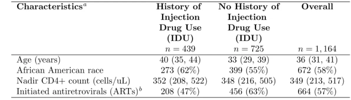
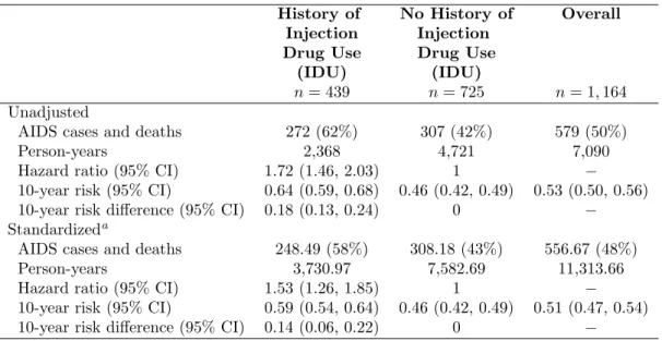
The 1,164 women were 58% African American, median age was 36 years, and median nadir CD4 count was 349 cells/µL at baseline (Table 3.1). At enrollment, 38% of women reported a history of IDU. During follow-up, 664 (57%) of women initiated ARTs. Women were followed for up to 10 years with a total of 7,090 person-years during which 579 (50%) developed AIDS or died, and 117 (10%) dropped out of the study. In analyses that did not account for covariates, women with a history of IDU had notably worse AIDS-free survival than women without a history of IDU (Figure 3.1). The estimated hazard ratio from the unadjusted Cox model was 1.72 (95% confidence interval (CI): 1.46, 2.03; Wald P value < 0.001), suggesting that the hazard of AIDS or death for those with a history of IDU was almost twice the hazard of those without a history of IDU (Table 3.2). We assessed the proportional hazards assumption graphically by examining whether the log cumulative hazard function estimates (See Figure 3.2) were approximately parallel. We also assessed this assumption statistically by inclusion of a product term between history of IDU and time in the Cox model, for which the Wald P value was 0.40. Neither graphical nor statistical assessment suggested a meaningful departure from proportional hazards.
We then obtained a standardized hazard ratio estimate from the IP-weighted Cox model, which involved two steps. In the first step, using separate logistic regression models, weights were estimated for the probability of exposure (i.e., history of IDU) and for the probability of not dropping out. For the exposure weights, we fit logistic regression models for both the numerator and denominator. The exposure model for the numerator had no covariates, while the exposure model for the denominator included age at baseline, race, and nadir CD4 count, as well as all pairwise interactions. Age and nadir CD4 were included as continuous variables using restricted quadratic splines with four knots placed at 5th, 35th, 65th, and 95thpercentiles
(Howe et al., 2011b). For the drop out weights, time was coarsened into months since baseline (Hernan et al., 2001). Then, using pooled logistic regression (D’Agostino et al., 1990), the drop out model for the numerator included only exposure (i.e., history of IDU) and time (using restricted quadratic splines), while the drop out model for the denominator included exposure, time (spline), age (spline), race, nadir CD4 count (spline), and ART initiation (time-varying), as well as all pairwise interactions. In the pooled logistic regression model, each person contributed up to 120 records and the weights were cumulatively multiplied for each person. The estimated weights ˆwi(t) had a mean of 1.01 (with a standard deviation of 0.76), and ranged from 0.43 to 12.43 (see Table 3.3). In the second step, the IP-weighted Cox model was fit by weighting participants by their estimated weights, with outcome time to AIDS or death, and history of IDU as the sole covariate.
We obtained the estimated survival functions from an IP-weighted Cox model with no covariates stratified by history of IDU. After standardization for confounding and drop out by IP weighting, survival curves showed an attenuated difference in AIDS-free survival compared to the survival curves without accounting for any covariates (Figure 3.1). Under certain assumptions discussed below, the dashed black curve can be interpreted as an estimate of the AIDS-free survival if (contrary to fact) everyone had a history of IDU at enrollment and did not drop out, while the solid black curve can be interpreted as an estimate of the AIDS-free survival if (contrary to fact) no one had a history of IDU at enrollment and everyone did not drop out (6, 7). The standardized hazard ratio from the IP-weighted Cox model was 1.53 (95% CI: 1.26, 1.85; Wald P value < 0.001) (Table 3.2). We again assessed the proportional hazards assumption graphically by examining whether the IP-weighted log cumulative hazard function estimates (See Figure 3.3) were approximately parallel. We also assessed this assumption statistically by inclusion of a product term between history of IDU and time, for which the Wald P value was 0.18. Neither graphical nor statistical assessment suggested a meaningful departure from proportional hazards. From the standardized survival curves, the ten-year risk of AIDS or death was 0.59 if (contrary to fact) everyone had a history of IDU at enrollment and 0.46 if (contrary to fact) no one had a history of IDU at enrollment. The 10-year risk difference was 0.14 (bootstrap 95% CI: 0.06, 0.22). For comparison, we also estimated a
covariate-adjusted hazard ratio by including history of IDU, age (spline), race, and nadir CD4 count (spline) directly in an unweighted Cox model. The covariate-adjusted hazard ratio estimate was 1.62 (95% CI: 1.35, 1.95; Wald P value < 0.001).
3.5 Discussion
IP-weighted Cox models and standardized survival curves were presented as methods to compare the timing of clinical events for two different exposure conditions under certain assumptions. We compare this method to the traditional Cox model and discuss assumptions and caveats below.
Although hazard ratio estimates from the IP-weighted and covariate-adjusted Cox model were comparable in the WIHS example above, the standardized (i.e., IP-weighted) method provides several potential benefits over the covariate-adjusted Cox model. First, the results from the standardized approach may be interpreted similar to results from a randomized trial with no drop out when only observational data is available (under certain assumptions discussed below). In particular, the estimated hazard ratio using the standardized approach can be interpreted the same as the (marginal) hazard ratio one would obtain in a randomized experiment such as a clinical trial where there is no confounding and no drop out. In con-trast, a covariate-adjusted Cox model hazard ratio does not necessarily equal the marginal hazard ratio because (even in the absence of unmeasured confounding) the Cox model is not collapsible for the hazard ratio parameter (Greenland, 1996). A regression model is said to be collapsible for a parameter (in this case, the hazard ratio) if the covariate-adjusted parameter is the same as the unadjusted parameter (Greenland et al., 1999b).
Second, the IP weighting approach yields standardized survival curve estimates. Although the hazard ratio is a common summary parameter to compare survival distributions between exposure groups, there are drawbacks to focusing inference on hazard ratios. For instance, the hazard ratio can be difficult to interpret, especially when trying to summarize the effect of a treatment or exposure (Hernan, 2010). Presenting estimated survival curves is an alternative to reporting hazard ratios that may be more interpretable because survival curves summarize
all information from baseline up to any time t. The IP-weighted approach leads to Kaplan-Meier type survival curve estimates that are standardized to the entire population under two different exposures at baseline while accounting for confounding by multiple covariates. A covariate-adjusted Cox model does not afford such survival curve estimates (Kaufman, 2010; Xie and Liu, 2005).
Third, the IP-weighted approach with drop out weights requires a weaker assumption about censoring than the covariate-adjusted Cox model (Hernan et al., 2000; Howe et al., 2011a; Kalbfleisch and Prentice, 2002). The adjusted Cox model assumes that the censoring hazard is independent of survival time conditional on being at risk, exposure, and baseline covariates, whereas the IP-weighted Cox model makes the weaker assumption that censoring is independent conditional on being at risk, exposure, baseline covariates, and time-varying covariates (Kalbfleisch and Prentice, 2002; Robins and Finkelstein, 2000). Specifically, if there are measured time-varying covariates predictive of censoring and survival time, the IP-weighted approach will yield consistent estimates of the marginal hazard ratio, while the covariate-adjusted Cox model estimator will not be consistent for the marginal or conditional hazard ratio (Hernan et al., 2000; Robins et al., 2000; Robins and Finkelstein, 2000).
Results using standardization by IP weights also have, in general, a different interpretation than results from an unadjusted Cox model. In particular, when exposure is confounded, the parameter of an unadjusted Cox model is a measure of association and will generally differ from the parameter of an IP-weighted Cox model (i.e., the marginal hazard ratio), which is a measure of effect (Robins et al., 2000). On the other hand, when exposure is unconfounded (e.g., as in randomized trials), the target parameter of both models is the marginal effect. In this case, drop out weights might still be employed to account for selection bias due to loss to follow-up (Hernan et al., 2013). Moreover, the use of IP drop out weights yields estimators that are more efficient (i.e., less variable) than those from an unadjusted Cox model even when there is no selection bias (Cole and Hernan, 2004; Robins and Finkelstein, 2000).
Estimation of the hazard ratio and survival curves using standardization by IP weights requires certain assumptions to yield valid inference about the exposure effect. In particular,