ECE-320

ECE-320: Linear Control Systems Homework 2

Due: Wednesday March 22 at 3:30 PM

1) For a system with transfer function

2

( )

2 3

a H s

s s

=

+ +

what is the range of values of aso that the absolute value of the steady state error for a unit step input is less than 0.2? What value of will produce a finite error for a unit ramp input? (Ans. ,3)

a

2.4< <a 3.6

2) For a system with transfer function

2

3 ( )

2 3

bs H s

s s

+ =

+ +

what is the range of values of b so that the absolute value of the steady state error for a unit ramp input is less than 0.1? What is the steady state error for a unit step input? (Ans.1.7< <b 2.3, 0)

3) An ideal second order system has the transfer function . The system specifications for a step input are as follows:

( ) o

G s

a) Percent Overshoot < 5%

b) Settling Time < 4 seconds (2% criteria) c) Peak Time < 1 second

Show the permissible area for the poles of G s_o( ) in order to achieve the desired response.

4) For a system with the following pole locations, estimate the settling time and determine the dominant poles

a) -1,-1,-4,-5 b) -4, -6, -6, -8 c) -1+j, -1-j, -2, -2 d) -3-2j, -3+2j, -4+j, -4-j

5) For the following transfer functions, determine • the characteristic polynomial

• the characteristic modes

• if the system is stable, unstable, or marginally stable

a) ( ) 1

( 2)( 10)

s H s

s s s

− =

+ +

b) ( ) ₂( ₂1)

( 1) ( 1

s s H s

s s s )

− =

+ + +

c) ( ) ₂ 1 ( 1)

H s

s s

= +

d)

2 2 1 ( )

( 1)( 2)( 1)

s H s

s s s

− =

− + +

e) ( ) ₂ 1

( 2)( 1

H s

s s

=

+ + )

6) For the transfer function

2

2 ( )

2 2

H s

s s

=

+ +

By computing the inverse Laplace transform show that the step response is given by

( ) ( ) tcos( ) ( ) tsin( ) ( )

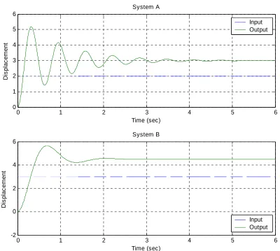
7) For systems A and B, with step responses shown in Figure 1, estimate • the percent overshoot

• the settling time

• the steady state error for the step input shown • the steady state error for a unit ramp input

0 1 2 3 4 5 6

0 1 2 3 4 5 6

System A

Di

s

p

la

c

e

m

e

nt

Time (sec)

Input Output

0 1 2 3 4 5 6

-2 0 2 4 6

System B

D

isp

la

ce

m

e

n

t

Time (sec)

Input Output

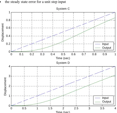
8) For systems C and D, with ramp responses shown in Figure 2, determine • the steady state error for the ramp input shown

• the steady state error for a unit step input

0 0.1 0.2 0.3 0.4 0.5 0.6 0.7 0.8 0.9 1

0 0.2 0.4 0.6 0.8 1

System C

D

isp

la

ce

m

e

n

t

Time (sec)

Input Output

0 0.5 1 1.5 2 2.5 3 3.5 4

0 1 2 3 4

System D

D

isp

la

ce

m

e

n

t

Time (sec)

Input Output

Figure 2. Ramp responses for systems C and D.

Answers for 7 and 8 (in no particular order, your approximations should be close, but they probably won't match.) 0,0,73%, 25%, 2, 3.5, -1, -1.2,1,0.16,∞,∞

9) For the following transfer functions, determine the static gain and the steady state output for a step input of amplitude 2.

1 2

2

3

2 ( )

1 1 ( )

2 1 ( )

( 1)( 3)

s G s

s s

s G s

s s G s

s s

+ =

+ + + =

+ − =

+

Preparation for Lab 3

As you undoubtedly recall, if we have a stable system with transfer function H s( ), and the input to the system isu t( )=Acos(ω θt+ ), then the steady state output is given by

( ) | ( ) | cos( ( ))

y t = H jω A ω θt+ + ∠H jω

This is really nothing more than a phasor relationship

[

][

]

Y = H jω ∠H jω U jω ∠U jω

j or

| | | ( ) || ( ) |

( ) ( )

Y H j U j

Y H j U

ω ω

ω ω

=

∠ = ∠ + ∠

10) Assume

( )

2

s H s

s

= +

a) If the input to this system is u t( )=3 cos(2 )t determine the steady state output. b) If the input to this system is u t( )=5sin(5t+10 )o determine the steady state output. (Ans. 2.12 cos(2t+45 ), 4.64 sin(5o t+31.8 )o )

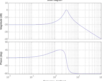
11) In addition to determining |H jω( ) | and ∠H jω( ) analytically, we can read these values from a Bode plot of the transfer function. Of course the magnitude portion of a Bode plot is in dB, and we need the actual amplitude |H jω( ) |. For the system with Bode plot given in Figure 5, determine the steady state output of this system if the input is

( ) 5sin(3 20 )o

u t = t+ and u t( )=5sin(2t+20 )o .

-40 -30 -20 -10 0 10

M

ag

ni

tud

e (

d

B

)

10-2 10-1 100 101 102

-90 -45 0 45 90

P

h

as

e (

d

eg

)

Bode Diagram

Frequency (rad/sec)

12) Now we want to use the Bode plot to identify the system. Let's assume the input to an unknown system is a sequence of sinusoids, u t( )= Acos(ω θt+ ) at different frequencies and different amplitudes. Once the transients have died out and the system is in steady state we measure the outputy t( ). We then have the following data:

( ) 4 cos(2 * 0.25 ) ( ) 0.089 cos(2 * 0.25 0.3 ) ( ) 4 cos(2 * 0.5 ) ( ) 0.092 cos(2 * 0.5 0.6 ) ( ) 4 cos(2 * ) ( ) 0.104 cos(2 * 1.4 ) ( ) 3cos(2 * 2 ) ( ) 0.178cos(2 * 2 6.2 ) ( ) 3cos(2 * 2.25 ) ( ) 0.32

o o o

o

u t t y t t

u t t y t t

u t t y t t

u t t y t t

u t t y t

π π π π π π π π π = = = = = = − = = −

= = 1cos(2 * 2.25 12.7 )

( ) 2 cos(2 * 2.4 ) ( ) 0.429 cos(2 * 2.4 28.1 ) ( ) 1cos(2 * 2.5 ) ( ) 0.424 cos(2 * 2.5 75.5 ) ( ) 1cos(2 * 2.6 ) ( ) 0.258cos(2 * 2.6 142.2 ) ( ) 2 cos(2 * 2.75 ) ( ) 0.218cos(2 * 2.75

o o o o

t

u t t y t t

u t t y t t

u t t y t t

u t t y t t

π π π π π π π π π − = = = = = =

= = 164.1 )

( ) 4 cos(2 *3 ) ( ) 0.207 cos(2 *3 171.9 ) ( ) 8cos(2 * 4 ) ( ) 0.115cos(2 * 4 176.9 ) ( ) 10 cos(2 *5 ) ( ) 0.075cos(2 *5 178.0 ) ( ) 10 cos(2 * 6 ) ( ) 0.047 cos(2 * 6 178.5 ) ( ) 10 cos(2 * 7 )

o o o o o

u t t y t t

u t t y t t

u t t y t t

u t t y t t

u t t y

π π π π π π π π π − = = − = = − = = − = = −

= ( ) 0.033cos(2 * 7 178.8 )

( ) 10 cos(2 *8 ) ( ) 0.024 cos(2 *8 180 ) o o

t t

u t t y t t

π π π = − = = − − − − − −

a) From this data, construct a table with theith input frequency f_i (in Hz), and the corresponding magnitude of the transfer function at that frequency , |H_i| |= H j( 2π f_i) |. Note that the amplitude of the input is changing. Note that we could also utilize the phase, but we don't need that for the systems we are trying to model.

b) Now we need to try and fit a transfer function to this data, i.e., determine a transfer function that will have the same Bode plot (at least the same magnitude portion). You will need to go though the following steps (you probably want to put this in an m-file...)

%

% I won't tell you how to do this again, so pay attention! %

% Enter the measured frequency response data %

w=2 *pi*[f₁ f₂ " f_n] % frequencies in radians/sec

H =[|H₁| |H₂| " |H_n |] % corresponding amplitudes of the transfer function %

% space them out logarithmically %

ww = logspace(log10(min(w)),log10(max(w)),1000); %

% next guess the parameters for a second order system, you will have to change these % to fit the data

%

omega_n = 20; zeta = 0.1; K = 0.05

HH = tf(K,[1/omega_n^2 2*zeta/omega_n 1]; %

% get the frequency response, this is one of many possible ways %

[M,P] = bode(HH,ww); M = M(:);

%

% Now plot them both on the same graph and make it look pretty %

semilogx(w,20*log10(H),'d',ww,20*log10(M),'-'); grid; legend('Measured','Estimated'); ylabel('dB'); xlabel('Frequency (rad/sec)');

title(['K = ' num2str(K) ', \omega_n = ' num2str(omega_n) ', \zeta = ' num2str(\zeta)]); %

% Note there are spaces between the single quote (') and the num2str function

If you have not screwed up, you should get the following graph:

100 101 102

-55 -50 -45 -40 -35 -30 -25 -20 -15 -10 -5

Frequency (rad/sec)

dB

K = 0.05, ω

n = 20, ζ = 0.1

Measured Estimated