ECE-320 Lab 6: State Variable Systems

1

ECE-320 Lab 6: State Variable Systems

In this lab you will look at different aspects of state variable systems and develop models in Simulink. Most of the Matlab calculations will be done for you.

PART A

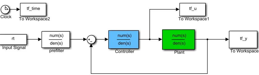
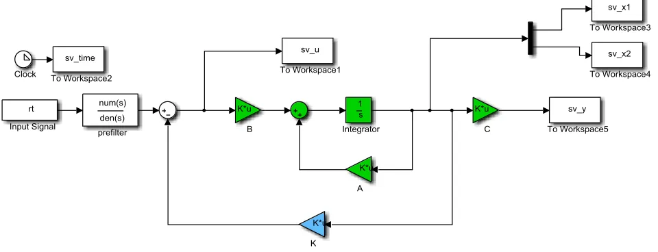
We can model an LTI system using either a transfer function model or a state variable model. In this part of the lab you will design a PI controller to control a system modelled using both of these methods, and hopefully become a bit more convinced that they are interchangeable. The file tf_model.slx is a simple control system using a transfer function model of the plant (shown in Figure 1), while sv_model.slx is a simple control system using a state variable model of the plant (shown in Figure 2.). Both of these models use the same controller and use the driver file tf_sv_driver.m.

The plant for this system can be represented using transfer functions as

2 3 ( ) 3 2 p s s s G s    

or using a state variable model





0 1 1

( ) ( )

2 3 0

y(t ( )

( )

) 1 0

x t u t

x x t t     _{ } _{ }       

You are to use sisotool to design a (continuous-time) PI controller and meet the following constraints:

1.0 sec, 20%, 12, 35

s PO kp ki

T    

Modify the controller in tf_sv_driver.m to use your controller and run the system. The results for both the transfer function model of the plant and the state variable model of the plant should be identical.

Include this graph in your memo, as well as the root locus plot for your PI controller and indicate the values of kp and ki in the caption of one of these figures.

2

Figure 2. State variable model of the plant.

PART B

In this part we will implement a state variable feeback control system using the same state variable model we used previously. Copy the file sv_model.slx to the file sv_feedback_model.slx, and modify this new file so it implements a state variable feedback model as shown in Figure 3.

Figure 3. State variable feedback system.

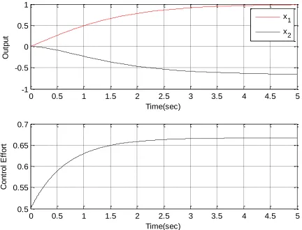
In the Matlab code sv_feedback_driver, the variable p indicates where the closed loop poles are placed. If you run this driver file with the default pole locations (-1 and -1.5) you should get a figure like that shown in Figure 4. Note that in this case the output is the first state (as determined by the vector C) and this C vector is used in the prefilter.

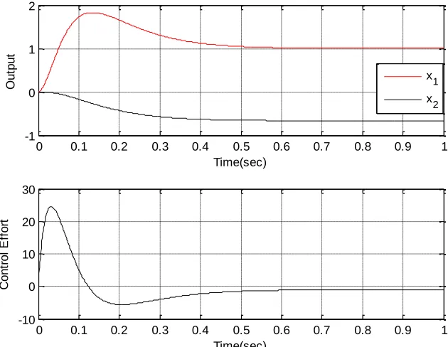
As mentioned in class, one of the benefits of state variable feedback is that if a system is controllable we can place the closed loop poles anywhere. Modify the code so the final time is 1.0 seconds, the closed loop poles are at -10 and -15, run the simulation, and include this figure in your memo. Then modify the code so the final time is 0.1 seconds, the closed loop poles are at -100 and -150, run the simulation, and

include this figure in your memo. You should notice that we can make the system respond more quickly

3 so the second state is the output. Run the simulation and include this figure in your memo (the second state should end up at 1.0.)

Figure 4. Result of state variable feedback with poles at -1 and -1.5 and the output is state one.

0 0.5 1 1.5 2 2.5 3 3.5 4 4.5 5

-1 -0.5 0 0.5 1

Time(sec)

O

u

tp

u

t

x₁ x₂

0 0.5 1 1.5 2 2.5 3 3.5 4 4.5 5

0.5 0.55 0.6 0.65 0.7

Time(sec)

C

o

n

tr

o

l

E

ff

o

4

PART C

Now we would like to modify our system so that it is a type one system and does not require a prefilter outside the feedback loop. Copy your file sv_feedback_model.slx to the file

sv_feedback_type1_model.slx and modify it so it looks like the system in Figure 5.

Figure 5. Type one state variable feedback system. Note an integrator is inside one of the feedback loops.

Run the file sv_feedback_type1_driver.m which computes all the required gains, and if the closedloop poles are at -10, -20, -30 (the default) you should get a figure like that in Figure 6. Modify the code so the output is state two, rerun the system, and include this figure in your memo.

Figure 6. Results of a type one state variable feedback system.

0 0.1 0.2 0.3 0.4 0.5 0.6 0.7 0.8 0.9 1

-1 0 1 2

Time(sec)

O

u

tp

u

t

x₁

x₂

0 0.1 0.2 0.3 0.4 0.5 0.6 0.7 0.8 0.9 1

-10 0 10 20 30

Time(sec)

C

o

n

tr

o

l

E

ff

o

5

PART D

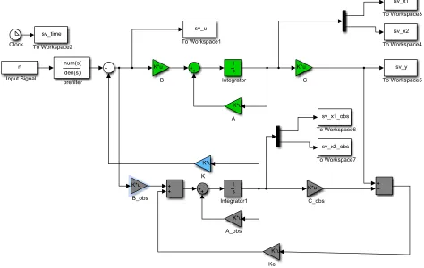
One of the biggest problems with state variable feedback systems is that we need to know the states. One way around this is to construct an observer which estimates the states of the system based on knowing the input and output of the system and the system dynamics. Copy your file

sv_feedback_model.slx to sv_feedback_observer_model.slx and modify it so it looks like the system shown in Figure 7. Note that in the observer you do not use the variables A, B, and C you used for the plant, but use A_obs, B_obs, and C_obs since in reality we only have an estimate of the true plant.

Figure 7. State variable feedback using an observer to estimate the states.

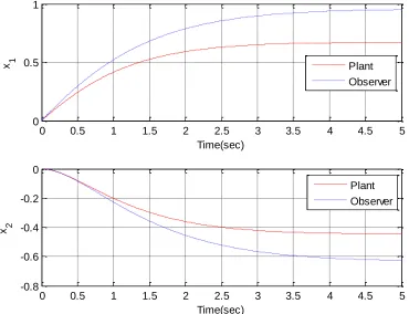
If you run the driver file sv_feedback_observer_driver.m you should get a plot like that in Figure 8. Note that for this system we have assumed that our model of the system (A_obs and B_obs) is off by a simple scaling. One thing you should notice about this plot is that our observer is not estimating the states very well. Part of this is because we assumed our model (A_obs and B_obs) had some pretty big errors, but the other part is that the poles of the observer are the same as the poles of the plant.What we really need is for the observer to converge to the estimated states faster than we expect the feedback system to converge. To do this, modify the code so that p_obs = p*3 (make the observer poles 3 times further from the origin than the state variable feedback poles, and reruns the system. Include this figure

in your memo. You should see the observer poles much closer to the real poles. However, you will also

see that the system does not reach the correct output due to our modelling errors.

6 is estimated much better, but the second state is worse. Now change C so the output is the second state and this is what goes to the observer. Now the observer should do much better for the second state than the first state.

Figure 8. Initial results using the observer in the state feedback model.

Now we want to make a small change in our system, so the state we send to the observer is not the state that is the output. To do this we will introduce a new variable Cy which is what we use to get the output. If we change our Simulink model it looks like that in Figure 9. Now the vector/matrix C indicates which combinations of states are going to the observer, and Cy indicates which combination of states that make up the output. Finally, you need to change the Matlab driver file so the prefiler is determined using Cy

instead of C_obs.

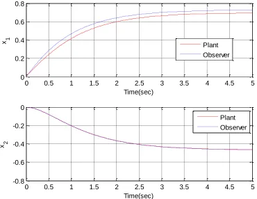
If we run this new system so the second state is going to the observer and the first state is the output, with the observer poles 10 time s further from the origin than the state feedback poles, we should get a figure like that in Figure 10. Include this figure in your memo.

Finally, there is nothing in how we constructed the observer that prevents us from sending more than one state to the observer (this would make more sense if we had a system with more than two states. With only two states I am really just messing with you…). Modify your code so both the first and second states are sent to the observer (C is not a 1 x 2 vector in this case!), the output is the second state, and the observer poles are 10 times further from the origin than the state feedback poles. Run the system

and include your figures in your memo.

0 0.5 1 1.5 2 2.5 3 3.5 4 4.5 5

0 0.5 1

Time(sec)

x 1 Plant

Observer

0 0.5 1 1.5 2 2.5 3 3.5 4 4.5 5

-0.8 -0.6 -0.4 -0.2 0

Time(sec)

x 2

7

Figure 9. State variable feedback system with C indicating states going to observer, and Cy indicating combination of states making up the output.

Figure 10. Results of observer system with state two going to the observer and state one the output state.

0 0.5 1 1.5 2 2.5 3 3.5 4 4.5 5

0 0.2 0.4 0.6 0.8

Time(sec)

x 1 _Plant

Observer

0 0.5 1 1.5 2 2.5 3 3.5 4 4.5 5

-0.8 -0.6 -0.4 -0.2 0

Time(sec)

x 2

8

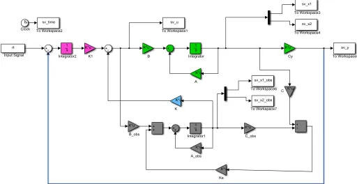
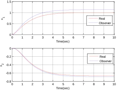
PART E

For this final part, we want to put everything together. You want to combine your observer and your type one Simulink files into a file sv_feedback_observer_types1.slx which should look like the system shown in Figure 10. If you run the program sv_feedback_observer_type1_driver.m you should get a figure like that in Figure 11. As you can see the output has not yet reached the correct final values. Modify the code so the observer poles are at -30 and -60, run the simulation, and include this graph in

your memo (the states should have converged.) Finally, assume both states are going to the observer and

the output is the second state (keep the observer poles at -30 and -60). Run this system and include this graph in your memo.

9

Figure 11. Initial results for type one state variable feedback system with an observer.

0 1 2 3 4 5 6 7 8 9 10

0 0.5 1 1.5

Time(sec)

x 1 Real

Observer

0 1 2 3 4 5 6 7 8 9 10

-0.8 -0.6 -0.4 -0.2 0

Time(sec)

x 2