Parsing Chinese Sentences with Grammatical Relations

Grammatical Relations

Weiwei Sun

Institute of Computer Science and Technology and Center for Chinese Linguistics ws@pku.edu.cn

Yufei Chen

Institute of Computer Science and Technology

yufei.chen@pku.edu.cn

Xiaojun Wan

Institute of Computer Science and Technology

wanxiaojun@pku.edu.cn

Meichun Liu

City University of Hong Kong Department of Linguistics and Translation

meichliu@cityu.edu.hk

We report our work on building linguistic resources and data-driven parsers in the grammatical relation (GR) analysis for Mandarin Chinese. Chinese, as an analytic language, encodes gram-matical information in a highly configurational rather than morphological way. Accordingly, it is possible and reasonable to represent almost all grammatical relations as bilexical dependencies. In this work, we propose to represent grammatical information using general directed dependency graphs. Both only-local and rich long-distance dependencies are explicitly represented. To create high-quality annotations, we take advantage of an existing TreeBank, namely, Chinese TreeBank (CTB), which is grounded on the Government and Binding theory. We define a set of linguistic rules to explore CTB’s implicit phrase structural information and build deep dependency graphs. The reliability of this linguistically motivated GR extraction procedure is highlighted by manual

Submission received: 23 November 2017; revised version received: 19 September 2018; accepted for publication: 19 November 2018.

evaluation. Based on the converted corpus, data-driven, including graph- and transition-based, models are explored for Chinese GR parsing. For graph-based parsing, a new perspective, graph merging, is proposed for building flexible dependency graphs: constructing complex graphs via constructing simple subgraphs. Two key problems are discussed in this perspective: (1) how to decompose a complex graph into simple subgraphs, and (2) how to combine subgraphs into a coherent complex graph. For transition-based parsing, we introduce a neural parser based on a list-based transition system. We also discuss several other key problems, including dynamic oracle and beam search for neural transition-based parsing. Evaluation gauges how successful GR parsing for Chinese can be by applying data-driven models. The empirical analysis suggests several directions for future study.

1. Introduction

Dependency grammar is a longstanding tradition that determines syntactic structures on the basis of word-to-word connections. It names a family of approaches to the lin-guistic analysis that all share a commitment to the typed relations between ordered pairs of words. Usually, dependencies represent various grammatical relations (GRs), which are exemplified in traditional grammars by the notions of subject, direct/indirect object, etc., and therefore encode rich syntactic information of natural language sentences in an explicit way. In recent years, parsing a sentence to a dependency representation has been well studied and widely applied to many Natural Language Processing (NLP) tasks, for example, Information Extraction and Machine Translation. In particular, the data-driven approaches have made great progress during the past two decades (K ¨ubler, McDonald, and Nivre 2009; Koo et al. 2010; Pitler, Kannan, and Marcus 2013; Chen and Manning 2014; Weiss et al. 2015; Dozat and Manning 2016). Various practical parsing systems have been built, not only for English but also for a large number of typologically different languages, for example, Arabic, Basque, Catalan, Chinese, Czech, Greek, Hungarian, Italian, and Turkish (Nivre et al. 2007).

Previous work on dependency parsing mainly focused on structures that can be represented in terms of directed bilexical dependency trees. Although tree-shaped graphs have several desirable properties from the computational perspective, they do not work well for coordinations, long-range dependencies involved in raising, control, as well as extraction, and many other complicated linguistic phenomena that go beyond the surface syntax. Some well-established and leading linguistic theories, such as Word Grammar (Hudson 1990) and Meaning-Text Theory (Mel’ˇcuk 2001), argue that more general dependency graphs are necessary to represent a variety of syntactic or semantic phenomena.

In this article, we are concerned with parsing Chinese sentences to an enriched deep dependency representation, which marks up a rich set of GRs to specify a linguistically-rich syntactic analysis. Different from the popularsurface1tree-based dependency rep-resentation, our GR annotations are represented as general directed graphs that express not only local but also various long-distance dependencies (see Figure 1 for example). To enhance the tree-shaped dependency representation, we borrow the key ideas under-lying Lexical Function Grammar (LFG) (Bresnan and Kaplan [1982], Dalrymple [2001]), a well-defined and widely-applied linguistic grammar formalism. In particular, GRs

浦东 近_{年 来} 颁_{布 实行 了 涉及 经济} 领_{域 的} 法_规性 _文件 Pudong recently issue practice involve economic field regulatory document

0 1 2 3 4 5 6 7 8 9 10 11

root root

comp _temp

temp subj

subj

prt prt

obj obj

subj*ldd

obj

nmod comp

relative nmod

Figure 1

An example:Pudong recently enacted regulatory documents involving the economic field. The symbol “*ldd” indicates long-distance dependencies; “subj*ldd” between the word “涉及/involve” and the word “文件/documents” represents a long-range subject-predicate relation. The arguments and adjuncts of the coordinated verbs, namely “颁布/issue” and “实行/practice,” are the separately yet distributively linked two heads.

can be viewed as the lexicalized dependency backbone of an LFG analysis that provides general linguistic insights.

To acquire a high-quality GR corpus, we propose a linguistically-motivated algo-rithm to translate a Government and Binding theory (GB) (Chomsky [1981], Carnie [2007]) grounded phrase structure treebank, namely, Chinese TreeBank (CTB) (Xue et al. [2005]) to a deep dependency bank where the GRs are explicitly represented. A manual evaluation highlights the reliability of our linguistically-motivated GR extraction algo-rithm: The overall dependency-based precision and recall are 99.17% and 98.87%. These numbers are calculated based on 209 sentences that are randomly selected and manually corrected. The automatically-converted corpus would be of use for a wide variety of NLP tasks, for example, parser training and cross-formalism parser evaluation.

By means of the newly created corpus, we study data-driven models for deep dependency parsing. The key challenge in building GR graphs is the range of relational flexibility. Different from the surface syntax, GR graphs are not constrained to trees. However, the tree structure is a fundamental consideration of the design for the majority of existing parsing algorithms. To deal with this problem, we proposegraph merging, an innovative perspective for building flexible representations. The basic idea is to decompose a GR graph into several subgraphs, each of which captures most but not necessarily the complete information. On the one hand, each subgraph issimpleenough to allow efficient construction. On the other hand, the combination of all subgraphs enables the whole target GR structure to be produced.

Based on this design, a practical parsing system is developed with a two-step architecture. In the first step, different graph-based models are applied to assign scores to individual arcs and various tuples of arcs. Each individual model is trained to target a unique type of subgraph. In the second step, a Lagrangian Relaxation-based joint decoder is applied to efficiently produce globally optimal GR graphs according to all graph-based models.

GR graphs. In particular, we consider the reachability property: In a given GR graph, every node is reachable from the same unique root. This property ensures that a GR graph can be successfully decomposed into a limited number of forests, which in turn can be accurately and efficiently built via tree parsing. Secondly, how can we merge subgraphs into one coherent structure in a principled way? The problem of finding an optimal graph that consistently combines the subgraphs obtained through individual models is non-trivial. We also treat this problem as an optimization problem and employ Lagrangian Relaxation to solve the problem.

Motivated by the recent successes of transition-based approaches to tree parsing, we also explore the transition-based models for building deep dependency structures. We utilize a list-based transition system that uses open lists for organizing partially processed tokens. This transition system is sound and complete with respect to directed graphs without self-loop. With reference to this system, we implement a data-driven parser with a neural classifier based on Long Short-Term Memory (LSTM) (Hochreiter and Schmidhuber [1997]). To improve the parsing quality, we look further into the impact of dynamic oracle and beam search on training and/or decoding.

Experiments on CTB 6.0 are conducted to profile the two types of parsers. Evalu-ation gauges how successful GR parsing for Chinese can be by applying data-driven models. Detailed analysis reveal some important factors that may possibly boost the performance. In particular, the following non-obvious facts should be highlighted:

1. Both the graph merging and transition-based parsers produce high-quality GR analysis with respect to dependency matching, although they do not use any phrase structure information.

2. When gold-standard POS tags are available, the graph merging model obtains a labeled f-score of 84.57 on the test set when coupled with a global linear scorer, and 86.17 when coupled with a neural model. Empirical analysis indicates the effectiveness of the proposed graph decomposition and merging methods.

3. The transition-based parser can be trained with either the dynamic oracle or the beam search method. According to our implementations, the dynamic oracle method performs better. Coupled with dynamic oracle, the transition-based parser reaches a labeled f-score of 85.51 when gold POS tags are utilized.

4. Gold-standard POS tags play a very important role in achieving the above accuracies. However, the automatic tagging quality of state-of-the-art Chinese POS taggers are still far from satisfactory. To deal with this problem, we apply ELMo (Peters et al. 2018), a contextualized word embedding producer, to obtain adequate lexical information. Experiments show that ELMo is extremely effective in harvesting lexical knowledge from raw texts. With the help of the ELMo vectors but not any POS tagging results, the graph merging parser achieves a labeled f-score of 84.90. This is a realistic set-up to evaluate how accurate the GR parsers could be for real-world Chinese Language Processing applications.

GR analysis and other syntactic/semantic analyses, including Universal Dependency, Semantic Role Labeling, and LFG’s f-structure, (2) the design of a new neural graph merging parser, (3) the design of a new neural transition-based parser, and (4) more comprehensive evaluations and analyses of the neural parsing models.

The implementation of the corpus conversion algorithm, a corpus visualization tool, and a set of manually labeled sentences are available athttp://www.aclweb.org/ anthology/attachments/P/P14/P14-1042.Software.zip. The implementation of the two neural parsers is available athttps://github.com/pkucoli/omg.

2. Background

2.1 Deep Linguistic Processing

Deep linguistic processing is concerned with NLP approaches that aim at modeling the complexity of natural languages in rich linguistic representations. Such approaches are typically related to a particular computational linguistic theory, including Combinatory Categorial Grammar (CCG) (Steedman [1996, 2000]), Lexical Functional Grammar (LFG) (Bresnan and Kaplan [1982], Dalrymple [2001]), Head-driven Phrase Structure Grammar (HPSG) (Pollard and Sag [1994]), and Tree-adjoining Grammar (TAG) (Joshi and Schabes [1997]). These theories provide not only the description of the syntactic structures, but also the ways in which meanings are composed, and thus parsing in these formalisms provides an elegant way to simultaneously obtain both syntactic and semantic analyses, generating valuable and richer linguistic information. Deep linguistic annotators and processors are strongly demanded in NLP applications, such as machine translation (Oepen et al. 2007; Wu, Matsuzaki, and Tsujii 2010) and text mining (Miyao et al. 2008). In general, derivations based on deep grammar formalisms may provide a wider variety of syntactic and semantic dependencies in more explicit details. Deep parses arguably contain the most linguistically satisfactory account of the deep dependen-cies inherent in many complicated linguistic phenomena, for example, coordination and extraction. Among the grammatical models, LFG and HPSG encode grammatical functions directly, and they are adequate for generating predicate–argument analyses (King et al. 2003; Flickinger, Zhang, and Kordoni 2012). In terms of CCG, Hockenmaier and Steedman (2007) introduced a co-indexing method to extract(predicate, argument) pairs from CCG derivations; Clark and Curran (2007a) also utilized a similar method to derive LFG-style grammatical relations. These bilexical dependencies can be used to approximate the corresponding semantic structures, such as logic forms in Minimal Recursion Semantics (Copestake et al. 2005).

In recent years, considerable progress has been made in deep linguistic processing for realistic texts. Traditionally, deep linguistic processing has been concerned with grammar development for parsing and generation. During the last decade, techniques for treebank-oriented grammar development (Cahill et al. 2002; Miyao, Ninomiya, and Tsujii 2005; Hockenmaier and Steedman 2007) and statistical deep parsing (Clark and Curran 2007b; Miyao and Tsujii 2008) have been well studied for English. Statistical models that are estimated on large-scale treebanks play an essential role in boosting the parsing performance.

2004; Briscoe and Carroll 2006; Clark and Curran 2007a; Bender et al. 2011), including C&C2 and Enju.3 If the interpretable predicate–argument structures are so valuable, then the question arises: Why cannot we directly build deep dependency graphs?

2.2 Data-Driven Dependency Parsing

Data-driven, grammar-free dependency parsing has received an increasing amount of attention in the past decade. Such approaches, for example, transition-based (Yamada and Matsumoto 2003; Nivre 2008) and graph-based (McDonald et al. 2005; McDonald, Crammer, and Pereira 2005) models have attracted the most attention in dependency parsing in recent works. Transition-based parsers utilize transition systems to derive dependency trees together with treebank-induced statistical models for predicting tran-sitions. This approach was pioneered by Yamada and Matsumoto (2003) and Nivre, Hall, and Nilsson (2004). Specifically, deep learning techniques have been successfully applied to enhance the parsing accuracy (Chen and Manning 2014; Weiss et al. 2015; Andor et al. 2016; Kiperwasser and Goldberg 2016; Dozat and Manning 2016).

Chen and Manning (2014) made the first successful attempt at incorporating deep learning into a transition-based dependency parser. A number of other researchers have attempted to address some limitations of their parser by augmenting it with additional complexity: Later it was enhanced with a more principled decoding algorithm, namely beam search, as well as a conditional random field loss objective function (Weiss et al. 2015; Watanabe and Sumita 2015; Zhou et al. 2015; Andor et al. 2016).

A graph-based system explicitly parameterizes models over substructures of a dependency tree, and formulates parsing as a Maximum Spanning Tree problem (McDonald et al. 2005). Similar to the transition-based approach, it also utilizes treebank annotations to train strong statistical models to assign scores to word pairs. Many re-searchers focus on developing principled decoding algorithms to resolve the Maximum Spanning Tree problem involved, for both projective (McDonald and Pereira 2006; Koo and Collins 2010) and non-projective structures (Koo et al. 2010; Kuhlmann 2010; Pitler, Kannan, and Marcus 2013). Deep learning has also been proved to be powerful for disambiguation and remained a hot topic in recent research (Kiperwasser and Goldberg 2016; Dozat and Manning 2016).

Kiperwasser and Goldberg (2016) proposed a simple yet effective architecture to implement neural dependency parsers. In particular, a bidirectional-LSTM (Bi-LSTM) is utilized as a powerfulfeature extractorto assist a dependency parser. Mainstream data-driven dependency parsers, including both transition- and graph-based ones, can apply useful word vectors provided by a Bi-LSTM to calculate scores. Following Kiperwasser and Goldberg (2016)’s experience, we implemented such a parser to evaluate the impact of empty categories on surface parsing.

Most research concentrated on surface syntactic structures, and the majority of existing approaches are limited to producing only trees. We notice several exceptions. Sagae and Tsujii (2008) and Henderson et al. (2013) individually introduced two tran-sition systems that can generate specific graphs rather than trees. Unfortunately, the two transition systems only cover 51.0% and 76.5%, respectively, of graphs in our data, highlighting the high complexity of our graph representation and the inadequacy of existing transition systems. McDonald and Pereira (2006) presented a graph-based

2http://svn.ask.it.usyd.edu.au/trac/candc/

parser that can generate dependency graphs in which a word may depend on multiple heads. Encouraged by their work, we study new data-driven models to build deep dependency structures for Mandarin Chinese.

2.3 Initial Research on Chinese Deep Linguistic Processing

In the last few years, study on deep linguistic processing for Chinese has been ini-tialized. Treebank annotation for individual formalisms is prohibitively expensive. To quickly construct deep annotations, corpus-driven grammar engineering has been de-veloped. Phrase structure trees in CTB have been semi-automatically converted to deep derivations in the CCG (Tse and Curran 2010), LFG (Guo, van Genabith, and Wang 2007), and HPSG (Yu et al. 2010) formalisms. To semi-automatically extract a large-scale HPSG grammar, Yu et al. (2010) defined a skeleton, including the structure of sign, grammatical principles, and schemata, based on which, the CTB trees are con-verted into HPSG-style trees. The treebank conversion under the CCG formalism is relatively easier. Tse and Curran (2010) followed the method proposed for English Penn Treebank (Hockenmaier and Steedman 2007) to process CTB. The main steps include (1) distinguishing head, argument, and adjunct, (2) binarizing CTB trees, and (3) re-defining syntactic categories. To more robustly construct f-structure for CTB trees, Guo, van Genabith, and Wang (2007) proposed a dependency-based model, which extracts functional information from dependency trees.

With the use of converted fine-grained linguistic annotations, successful English deep parsers, such as C&C (Clark and Curran 2007b) and Enju (Miyao and Tsujii 2008), have been evaluated on the Chinese annotations (Yu et al. 2011; Tse and Curran 2012). Although the discriminative learning architecture of both C&C and Enju parsers makes them relatively easy to be adapted to solve multilingual parsing, their performance on Chinese sentences is far from satisfactory. Yu et al. (2011) and Tse and Curran (2012) analyze the challenges and difficulties in Chinese deep parsing. In particular, some language-specific properties account for a large number of errors.

3. Representing Deep Linguistic Information Using Dependency Graphs

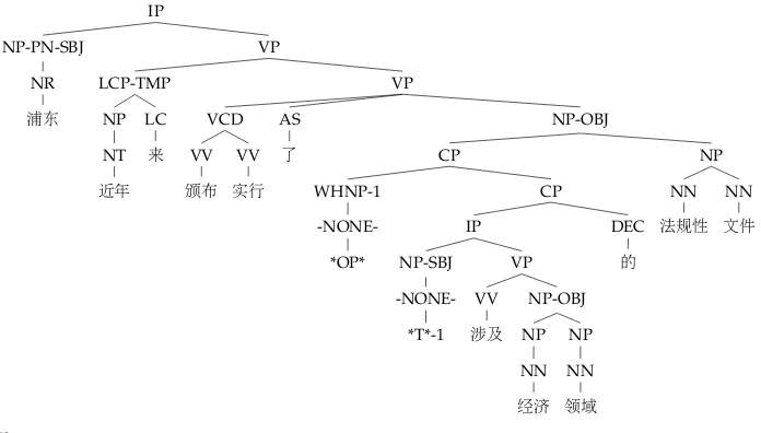
In this section, we discuss the construction of the GR annotations. Basically, the an-notations are automatically converted from a GB-grounded phrase structure treebank, namely CTB. Conceptually, this conversion is similar to the conversions from CTB struc-tures to representations in deep grammar formalisms (Xia 2001; Guo, van Genabith, and Wang 2007; Tse and Curran 2010; Yu et al. 2010). However, our work is grounded in GB, which is the linguistic basis of the construction of CTB. We argue that this theoretical choice makes the conversion process more compatible with the original annotations and therefore more accurate. We use directed graphs to explicitly encode bilexical dependen-cies involved in coordination, raising/control constructions, extraction, topicalization, and many other complicated phenomena. Figure 2 shows the original CTB annotation of the sentence in Figure 1.

3.1 Linguistic Basis

IP

VP

VP

NP-OBJ

NP NN 文件 NN 法_规性 CP

CP

DEC 的 IP

VP NP-OBJ

NP NN

领域

NP NN 经济

VV

涉及

NP-SBJ

-NONE-*T*-1 WHNP-1

-NONE-*OP* AS 了 VCD

VV 实行 VV

颁_布

LCP-TMP LC

来 NP NT 近_年 NP-PN-SBJ

NR

浦东

Figure 2

The original CTB annotation of the running example.

appear. In highlyconfigurationallanguages, for example, Chinese, however, the grammatical function of a phrase is heavily determined by its constituent structure position. Dominant Chomskyan theories, including GB, have defined GRs as configurations at phrase structures. Following this principle, CTB groups words into constituents through the use of a limited set of fundamental grammatical functions. For example, one bracket represents only one grammatical relation in CTB, providing phrase structure annota-tions with specificaannota-tions of particular grammatical funcannota-tions. Transformational grammar utilizes empty categories to represent long-distance dependencies. In CTB, traces are pro-vided by relating displaced linguistic material to where it should be interpreted seman-tically. By exploiting configurational information, traces, and functional tag annotations, GR information can hopefully be derived from CTB trees with high accuracy.

3.2 The Extraction Algorithm

Our treebank conversion algorithm borrows key insights from LFG. LFG posits two levels of representation: c(onstituent)-structure and f(unctional)-structure minimally. C-structure is represented by phrase structure trees, and captures surface syntactic configurations such as word order, whereas f-structure encodes grammatical functions. It is easy to extract a dependency backbone that approximates basic predicate– argument–adjunct structures from f-structures. The construction of the widely used PARC DepBank (King et al. 2003) is a good example.

LFG relates c-structure and f-structure through f-structure annotations, which com-positionally map every constituent to a corresponding f-structure. Borrowing this key idea, we translate CTB trees to dependency graphs by first augmenting each con-stituency with f-structure annotations, then propagating the head words of the head or conjunct daughter(s) upwards to their parents, and finally creating a dependency graph. The details are presented step-by-step as follows:

IP

VP ↓=↑

VP ↓=↑

NP ↓=(↑OBJ)

NP ↓=↑

NN ↓=↑

文件

NN ↓∈(↑NMOD)

法_规性

CP ↓∈(↑REL)

DEC ↓=↑

的

IP ↓=(↑COMP)

VP ↓=↑

NP ↓=(↑OBJ)

NN ↓=↑ 领_域 NP

↓∈(↑NMOD)

NN ↓=↑ 经济

VV ↓=↑

涉及

NP ↓=(↑SUBJ)

-NONE-*T* AS

↓=(↑PRT) 了 VCD

↓=↑

VV ↓∈↑ 实行

VV ↓∈↑ 颁_布 LCP

↓∈(↑TMP)

LC ↓=↑

来 NP ↓=(↑COMP)

NT ↓=↑

近_年

NP ↓=(↑SUBJ)

NR

浦东

Figure 3

The original CTB annotation augmented with LFG-like functional annotations of the running example.

start to extract GRs. We slightly modify their method to enrich a CTB tree with f-structure annotations: Each node in a resulting tree is annotated with one and only one corresponding equation (see Figure 3 for an example). Comparing the original and enriched annotations, we can see that the functionality of this step is to explicitly represent and regulate grammatical functions4for every constituent. We enrich the CTB trees with function information by using the conversion tool5that generated the Chinese data sets for the CoNLL 2009 Shared Task on multilingual dependency parsing and semantic role labeling.

3.2.2 Beyond CTB Annotations: Tracing More.Natural languages do not always interpret linguistic materials locally. In order to obtain accurate and complete GR, predicate– argument, or logical form representations, a hallmark of deep grammars is that they usually involve a non-local dependency resolution mechanism. CTB trees utilize empty categories and co-indexed materials to represent long-distance dependencies. An empty category is a nominal element that does not have any phonological content and is therefore unpronounced. There are two main types of empty categories: null pronounce and trace, and each type can be further classified into different subcategories. Two kinds of anaphoric empty categories, that is, big PRO and trace, are annotated in CTB. Theoretically speaking, only trace is generated as the result ofmovementand therefore annotated with antecedents in CTB. We carefully checked the annotation and found that considerable amounts of antecedents are not labeled, and hence a large sum of important non-local information is missing. In addition, because the big PRO is also

anaphoric, it is possible to find co-indexed components sometimes. Such non-local information is also valuable in marking the dependency relation.

Beyond CTB annotations, we introduce a number of phrase structure patterns to extract more non-local dependencies. The method heavily leverages linguistic rules to exploit structural information. We take into account both theoretical assumptions and analyzing practices to enrich co-indexation information according to phrase struc-ture patterns. In particular, we try to link an anaphoric empty category e with its c-commonders if no non-empty antecedent has already been co-indexed withe. Because the CTB is influenced deeply by the X-bar syntax, which highly regulates constituent analysis, the number of linguistic rules we have is quite modest. For the development of conversion rules, we used the first 9 files of CTB, which contain about 100 sentences. Readers can refer to the well-documented Perl script for details (see Figure 3 for an example). The noun phrase “法_规性_{文件/regulatory documents” is related to the trace} “*T*.” This co-indexation is not labeled in the original annotation.

3.2.3 Passing Head Words and Linking Empty Categories. Based on an enriched tree, our algorithm propagates the head word of the head daughter upwards to their parents, linking co-indexed units, and finally creating a GR graph. The partial result after head word passing of the running example is shown in Figure 4. There are two differences in the head word passing between our GR extraction and a “normal” dependency tree extraction. First, the GR extraction procedure may pass multiple head words to their parent, especially in a coordination construction. Secondly, long-distance dependencies are created by linking empty categories and their co-indexed phrases.

The coding of long-distance dependency relations is particularly important for processing grammatical relations in Chinese. Compared to English, Chinese allows more flexibility in word order and a wider range of “gap-and-filler” relations. Among the common long-distance dependencies such as co-referential indexing, cleft-focus, prepositional phrase, and coordination, relativization in Chinese is of particular interest. Chinese relativization is structurally head-final, with the relative clause, marked by de的(the grammatical marker of nominal modifier), occurring before the head noun. The head noun may hold any kind of semantic relation with the proceeding relative

IP{颁_布,实行}

VP{颁_布,实行}

VP{颁_布,实行}

NP{_文件}

NP{文件} CP{的}

DEC{_的} IP{_涉及}

VP{涉及} NP{文件*ldd}

AS{_了} VP{颁_布,实行} LCP{来}

NP{_浦东}

Figure 4

Table 1

Manual evaluation of 209 sentences.

Precision Recall F1

Unlabeled 99.48 99.17 99.32

Labeled 99.17 98.87 99.02

clause. In other words, Chinese relative structure will have the “gap” occurring before the “filler” and there is little restriction on the semantic roles of the relativized head noun. Chinese-specific structural peculiarities may give rise to unexpected difficulties in sentence processing. Applying an augmented version of dependency notations, our system is able to handle such complicated issues in processing Chinese sentences.

3.3 Manual Evaluation

To have a precise understanding of whether our extraction algorithm works well, we have selected 20 files that contain 209 sentences in total for manual evaluation. Linguis-tic experts carefully examine the corresponding GR graphs derived by our extraction algorithm and correct all errors. In other words, a gold-standardGR annotation set is created. The measure for comparing two dependency graphs is precision/recall of GR tokens, which are defined ashwh,wd,lituples, wherewhis the head,wdis the dependent, andl is the relation. Labeled precision/recall (LP/LR) is the ratio of tuples correctly identified by the automatic generator, while unlabeled precision/recall (UP/UR) is the ratio regardless ofl. F-score is a harmonic mean of precision and recall. These measures correspond to attachment scores (LAS/UAS) in dependency tree parsing. To evaluate our GR parsing models that will be introduced later, we also report these metrics.

The overall performance is summarized in Table 1. We can see that the automatic GR extraction achieves relatively high performance. There are two sources of errors in treebank conversion: (1) inadequate conversion rules and (2) wrong or inconsistent original annotations. During the creation of the gold-standard corpus, we find that rule-based errors are mainly caused by complicated unbounded dependencies and the lack of internal structure for some phrases. Such problems are very hard to solve through rules only, if even possible, since original annotations do not provide sufficient information. The latter problem is more scattered and unpredictable, which requires manual correction.

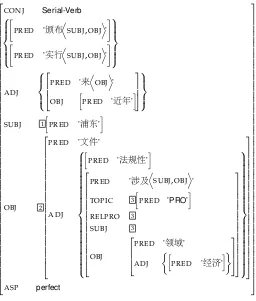
3.4 Comparing to the De Facto LFG Analysis

IP

VP ↓=↑

VP ↓=↑

NP ↓=(↑OBJ)

NP ↓=↑

NN ↓=↑

文件

NN ↓∈(↑ADJ)

法_规性

CP ↓∈(↑ADJ)

DEC (↑TOPIC PRED)=’PRO’

(↑TOPIC)=(↑SUBJ) (↑RELPRO)=(↑TOPIC)

的

IP ↓=↑

VP ↓=↑

NP ↓=(↑OBJ)

NN ↓=↑ 领_域 NP ↓∈(↑ADJ)

NN ↓=↑ 经济

VV ↓=↑

涉及

AS (↑ASP)=perfect

了 VCD

↓=↑

VV ↓∈↑ 实行

VV ↓∈↑ 颁_布 LCP ↓∈(↑ADJ)

LC ↓=↑ 来 NP ↓=(↑OBJ)

NT ↓=↑

近_年

NP ↓=(↑SUBJ)

NR

浦东

Figure 5

A de facto c-structure of the running example. The c-structure is augmented by a number of functional schemata.

corresponding functional description. Finally, we solve the simultaneous equations of these functional descriptions and then construct the minimal f-structure that satisfies them. Figure 6 shows the f-structure of the running sentence. According to the linguistic assumptions under LFG, this f-structure is more linguistically universal and has a tighter relationship with semantics.

Comparing the two trees in Figures 3 and 5, we can see that most functional schemata are similar. There are two minor differences between the LFG and our GR analysis.

1. LFG utilizes functional schemata that are assigned to phrase structures rather than empty categories to analyze a number of complex linguistic phenomena. Therefore, in the standard LFG c-structure tree, there is no “-NONE- *T*”-style terminals. Instead, specific constructions or function words take the responsibility. Our corpus is based on the original annotations of CTB, which is based on the GB theory. As a result, our grammatical function-augmented trees include unpronounced nodes, and there are not many functional schemata associated with constructions or function words.

                                                 CONJ Serial-Verb         

PRED ’颁布

D

SUBJ,OBJE’

PRED ’实行

D

SUBJ,OBJE’

         ADJ        

PRED ’来

D OBJ E ’ OBJ h

PRED ’近年’

i         SUBJ 1 h

PRED ’浦东’

i OBJ 2                      

PRED ’文件’

ADJ                                      h

PRED ’法规性’

i               

PRED ’涉及

D

SUBJ,OBJE’

TOPIC 3

h

PRED ’PRO’i

RELPRO 3 SUBJ 3 OBJ   

PRED ’领域’

ADJ

h

PRED ’经济’

i                                                                              ASP perfect                                                  Figure 6

A de facto f-structure of the running example.

Some annotations may be different due to theoretical considerations. Take relative clause for example. The analysis in Figures 5 and 6 is based on the solution provided by Dalrymple (2001) and Bresnan (2001). The predicate–argument relation between “涉及/involve” and “文件/document” is not included because LFG treats this as an anaphoric problem. However, we argue that this relation is triggered by the function word de “的” as a marker of modification and is therefore put into our GR graph. Another motivation of this design is to let our GR graph represent more semantic information. We will continue to discuss this topic in the next subsection.

3.5 Comparing to Other Dependency Representations

In this section, we consider the differences between our GR representation and other popular dependency-based syntactic and semantic analyses. Figure 7 visualizes four types of cross-representation annotations assigned to the sentence in Figure 1:

1. our GR graph,

2. the CTB-dependency tree,

3. the Universal Dependency, and

Two of the dependency representations are based on tree structures that are repre-sentative of Chinese Language Processing. Both are converted from CTB by applying heuristic rules. The CTB-dependency tree is the result of transformation introduced by Xue (2007), with a constituency-to-dependency transformation algorithm that explores the implicit functional information of CTB. This dependency corpus is used by the

浦东 近年 来 颁_{布 实行 了 涉及 经济} 领_{域 的} 法_规性 _文件

root root

comp temp

temp subj

subj

prt prt

obj obj

subj*ldd

obj nmod comp

relative nmod

(a) The GR graph.

浦东 近年 来 颁_{布 实行 了 涉及 经济} 领_{域 的} 法_规性 _文件 root

comp temp

subj

cjt prt

obj

obj nmod comp

relative nmod

(b) The CTB-dependency.

浦东 近_{年 来} 颁_{布 实行 了 涉及 经济} 领_{域 的} 法_规性 _文件 root

case advmod:loc nsubj

compound:vc aux:asp

dobj

dobj compound:nn

mark

acl:relcl

compound:nn

(c) Universal dependency.

浦东 近_{年 来} 颁_{布 实行 了 涉及 经济} 领_{域 的} 法_规性 _文件 ArgM-TMP

ArgM-TMP Arg0

Arg1

Arg0

Arg1

Arg1

Arg0

(d) PropBank-style Semantic role labeling. Figure 7

CoNLL 2009 shared task. Because this transformation algorithm is proposed by the developer and maintainer, we call it CTB-dependency. The Universal Dependency6 corpus for Chinese is also based on CTB but with different constituency-to-dependency transformation rules. Both the language- and treebank-specific properties and compa-rability to resources of other languages are considered. The last representation is mo-tivated by semantic processing and the dependencies reflect basic predicate–argument structures of verbs. The annotations are from Chinese PropBank (Xue and Palmer 2009), a sister resource to CTB. The head words are verbs or their normalizations, while the dependent words take semantic roles pertaining to the related verbs.

It can be clearly seen that compared to the tree-shaped dependency analysis, our GR representation represents much more syntactic information though more general graphs. In addition, the syntactic information of our analysis is more transparent with respect to (compositional) semantics. This property is highlighted by the structural parallelity between our GR graphs and the semantic role labeling results.

• Take, for example, the serial verb construction, a special type of

coordination (颁布实行了“issued-practiced”). According to the properties of distributive features, the shared subject, object, and aspect marker hold the same grammatical relations regarding bothconjuncts. Limited by the single-head constraint, a dependency tree cannot represent all of these dependencies in an explicit way.

• Take the relative clause construction for another example (涉及经济领域的

法_规性_{文件“the regulatory document that involves economic field”).} There is a long-distance predicate–argument dependency between “涉 及/involve” and “文件/document.” The addition of this dependency to a tree will bring in a cycle for the CTB-dependency analysis. The Universal Dependency analysis includes this dependency, because its annotations are driven by not only syntax but also semantics. Nevertheless, the related label lacks the information that a subject is displaced.

3.6 A Quantitative Analysis

In the previous two subsections, we presented a phenomenon-by-phenomenon com-parison to show the similarity and dissimilarity between our GR analysis and other syntactic/semantic analyses, for example, Universal Dependency, Semantic Role Label-ing, and LFG’s f-structure. In this subsection, we present a quantitative analysis based on overall statistics of the derived dependency corpus and a quantitative comparison with the CTB-dependency corpus. Table 2 shows how many dependencies are shared by both representations. The majority of grammatical relations involve local dependencies, and therefore the intersection of both representations are quite large. Nevertheless, a considerable number of dependencies of the GR representation do not appear in the tree representations. In principle, the GR representation removes semantically irrelevant dependencies, and thus it contains fewer arcs. Figure 8 summarizes the distribution of governable and non-governable GRs with respect to the tree and graph corpora.

Table 2

The distribution of the unlabeled dependencies. The “Tree” and “Graph” rows indicate how many dependencies, that is, arcs, in total are included by the CTB-dependency and our graph representations. Sentences are selected from CTB 6.0 and have been used by the CoNLL 2009 shared task. “Graph∩Tree” means the dependencies in common; “Graph–Tree” means the dependencies that appear in the GR graphs but not the CTB-dependency trees; “Tree–Graph” means the dependencies that appear in the CTB-dependency trees but not the GR graphs.

#Arc

Tree 731,833

Graph 669,910

Graph∩Tree 554,240 Graph–Tree 115,670 Tree–Graph 177,593

0 5 10 15 20 25

ADV AMODCOMP LOC NMOD OBJ SBJ TMP

%

Tree Graph

Figure 8

The distribution of the dependency relations.

4. Graph-Based Parsing via Graph Merging

4.1 The Proposal

The key proposal of this work is to construct a complex structure via constructing simple partial structures. Each partial structure is simple in the sense that it allows efficient construction. To construct each partial structure, we can employ mature parsing techniques. To obtain the final target output, it requires the total of all partial structures as they enable the whole target structure to be produced. This article aims to exemplify the above idea by designing a new parser for obtaining GR graphs. Take the GR graph in Figure 1 for example. It can be decomposed into two tree-like subgraphs, as shown in Figure 9. If we can parse the sentence into subgraphs and combine them in a principled way, we are able to obtain the original GR graph.

浦东 近_{年 来} 颁_{布 实行 了 涉及 经济} 领_{域 的} 法_规性 _文件

root

root comp

comp temp subj

prt

obj

temp

subj

prt

obj

subj[inverse] obj

nmod

obj nmod comp

relative nmod

nmod

Figure 9

A graph decomposition for the GR graph in Figure 1. The two subgraphs are shown on two sides of the sentence, respectively. The subgraph on the upper side of the sentence is exactly a well-formed tree, while the one on the lower side is slightly different. The edge from the word “文件/document” to “涉及/involve” is tagged “[inverse]” to indicate that the direction of the edge in the subgraph is in fact opposite to that in the original graph.

which allows us to produce coherent structures as outputs. The techniques we devel-oped to solve the two problems are demonstrated in the following sections.

4.2 Decomposing GR Graphs

4.2.1 Graph Decomposition as Optimization.Given a sentences=w0w1w2· · ·wnof length

n(where w0 denotes the virtual root), a vectoryyyof lengthn(n+1) is used to denote

a graph on the sentence. Indicesi and j are then assigned to index the elements in the vector,yyy(i,j)∈ {0, 1}, denoting whether there is an arc from wi to wj (0≤i≤n, 1≤j≤n).

Given a graphyyy, there may bemsubgraphsyyy1, . . . ,yyym, each of which belongs to a specific class of graphsG_k(k=1, 2,· · ·,m). Each class should allow efficient construc-tion. For example, we may need a subgraph to be a tree or a non-crossing dependency graph. The combination of allyyykgives enough information to constructyyy. Furthermore, the graph decomposition procedure is utilized to generate training data for building submodels. Therefore, we hope each subgraphyyykis informative enough to train a good scoring model. To do so, for eachyyyk, we define a score functionsk that indicates the “goodness” ofyyyk. Integrating all ideas, we can formalize graph decomposition as an optimization problem,

max.P ksk(yyyk) s.t. yyyibelongs toGi

P

kyyyk(i,j)≥yyy(i,j),∀i,j

The last condition in this optimization problem ensures that all edges inyyy appear at least in one subgraph.

For a specific graph decomposition task, we should define good score functionssk and graph classesG_k, according to key properties of the target structureyyy.

an independent connected component. This property allows a GR graph to be decom-posable into a limited number oftree-likesubgraphs. By tree-like, we mean that if we treat a graph on a sentence as undirected, it is either a tree, or a subgraph of some tree on the sentence. The advantage of tree-like subgraphs is that they can be effectively built by adapting data-driven tree parsing techniques. Take the sentence in Figure 1, for example. For every word, there is at least one path linking the virtual root and the target word. Furthermore, we can decompose the graph into two tree-like subgraphs, as shown in Figure 9. In such decomposition, one subgraph is exactly a tree, and the other is very close to a tree.

In practice, we restrict the number of subgraphs to 3. The reasoning is that we use one tree to capture long distance information and the other two to capture coordination information.7 _{In other words, we decompose each given graphyyy into three tree-like}

subgraphsggg1,ggg2, andggg3for each subgraph to carry important information of the graph

as well as cover all edges inyyy. The optimization problem can be written as

max.s1(ggg1)+s2(ggg2)+s3(ggg3)

s.t. ggg1,ggg2,ggg3are tree-like

ggg1(i,j)+ggg2(i,j)+ggg3(i,j)≥yyy(i,j),∀i,j

Scoring a Subgraph. We score a subgraph in a first order arc-factoredway, which first scores the edges separately and then adds up the scores. Formally, the score function issk(ggg)=Pωk(i,j)gggk(i,j) (k=1, 2, 3) whereωk(i,j) is the score of the edge fromitoj. Under this score function, we can use the Maximum Spanning Tree (MST) algorithm (Chu and Liu 1965; Edmonds 1967; Eisner 1996) to decode the tree-like subgraph with the highest score.

After the score function is defined, extracting a subgraph from a GR graph works in the following way: We first assign heuristic weightsω_k(i,j) (1≤i,j≤n) to the potential edges between all the pairs of words, then compute a best projective treegggkusing the Eisner’s Algorithm (Eisner 1996):

gggk=arg max

ggg sk(ggg)=arg maxggg X

ω_k(i,j)ggg(i,j).

gggkis not exactly a subgraph ofyyy, because there may be some edges in the tree but not in the graph. To guarantee a meaningful subgraph of the original graph, we add labels to the edges in trees to encode necessary information. We labelgggk(i,j) with the original label, ifyyy(i,j)=1; with the original label appended by “∼R” ifyyy(j,i)=1; with “None” else. With this labeling, we can have a functiont2gto transform the extracted trees into tree-like graphs.t2g(gggk) is not necessarily the same as the original graphyyy, but it must be a subgraph of it.

Three Variations of Scoring. With different weight assignments, different trees can be extracted from a graph, obtaining different subgraphs. We devise three variations of

weight assignment:ω₁,ω₂, andω₃. Each of theω’s consists of two parts. One is shared by all, denoted byS, and the other is different from each other, denoted byV. Formally,

ω_k(i,j)=S(i,j)+Vk(i,j) (k=1, 2, 3 and 1≤i,j≤n).

Given a graphyyy,Sis defined asS(i,j)=S1(i,j)+S2(i,j)+S3(i,j)+S4(i,j), where

S1(i,j)=

(

w1 ifyyy(i,j)=1 oryyy(j,i)=1

0 else (1)

S2(i,j)=

(

w2 ifyyy(i,j)=1

0 else (2)

S3(i,j)=w3(n− |i−j|) (3)

S4(i,j)=w4(n−lp(i,j)) (4)

In the definitions above,w1,w2,w3, andw4 are coefficients, satisfyingw1 w2 w3, andlpis a function ofiandj.lp(i,j) is the length of shortest path fromitojthat either

iis a child of an ancestor ofjorjis a child of an ancestor ofi. That is to say, the paths are in the formi←n1← · · · ←nk→jori←n1→ · · · →nk→j. If no such path exists, thenlp(i,j)=n. The reasoning behind the design is illustrated below.

S1 indicates whether there is an edge betweeniandj, and it is meant for optimal effect; S2 indicates whether the edge is fromi to j, and we want the edge with the correct

direction more likely to be selected;

S3 indicates the distance between i and j, and we like the edge with short distance

because it is easier to predict;

S4 indicates the length of certain types of path between i and j that reflects

c-commanding relationships, and the coefficient remains to be tuned.

The score V is meant to capture different information from the GR graph. In GR graphs, we have an additional piece of information (as denoted as “*ldd” in Figure 1) for long-distance dependency edges. Moreover, we notice that conjunction is another important structure, which can be derived from the GR graph. Assume that we tag the edges relating to conjunctions with “*cjt.” The three variation scores, that is,V1,V2, and V3, reflect long distance and the conjunction information in different ways.

V1.First for edgesyyy(i,j) whose label is tagged with *ldd, we assignV1(i,j)=d.8

When-ever we come across a parentpwith a set of conjunction childrencjt1,cjt2,· · ·,cjtn, we look for the rightmost childgc1rof the leftmost child in conjunctioncjt1, and adddto

eachV1(p,cjt1) andV1(cjt1,gc1r). The edges in conjunction to which additionald’s are added are shown in blue in Figure 10.

V2. Different from V1, for edges yyy(i,j) whose label is tagged with *ldd, we assign V2(j,i)=d. Then for each conjunction structure with a parentp and a set of

conjunc-tion childrencjt1,cjt2,· · ·,cjtn, we find the leftmost childgcnl of the rightmost child in

wp ... wc1 ... wgc2 ... wgc1 ... wc2 ... wl X*cjt

X*cjt X*cjt

X*ldd

Figure 10

Examples to illustrate the additional weights.

conjunctioncjtn, and adddto eachV2(p,cjtn) andV2(cjtn,gcnl). The concerned edges in conjunction are shown in green in Figure 10.

V3.We do not assignd’s to the edges with tag *ldd. For each conjunction with parent pand conjunction childrencjt1,cjt2,· · ·,cjtn, we adddtoV3(p,cjt1),V3(p,cjt2),· · ·, and V3(p,cjtn).

4.2.3 Lagrangian Relaxation with Approximation.As soon as we identify three treesggg1,ggg2,

andggg3, there are three subgraphsggg1 =t2g(ggg1),ggg2=t2g(ggg2), andggg3 =t2g(ggg3). As stated

above, each edge in a graphyyyneeds to be covered by at least one subgraph, and the goal is to maximize the sum of the edge weights of all trees. Note that the inequality in the constrained optimization problem above can be replaced by a maximization, written as

max.s1(ggg1)+s2(ggg2)+s3(ggg3)

s.t. ggg1,ggg2,ggg3are trees

max{t2g(ggg1)(i,j),t2g(ggg2)(i,j), t2g(ggg3)(i,j)}=yyy(i,j),∀i,j

wheresk(gggk)=Pωk(i,j)gggk(i,j)

Letgggm=max{t2g(ggg1),t2g(ggg2),t2g(ggg3)}, and by max{ggg1,ggg2,ggg3}we mean to take the

maximum of three vectors pointwisely. The Lagrangian of the problem is

L(ggg1,ggg2,ggg3;u)=s1(ggg1)+s2(ggg2)+s3(ggg3)+u>(gggm−yyy)

whereuis the Lagrangian multiplier. Then the dual is

L(u)= max ggg1,ggg2,ggg3

L(ggg1,ggg2,ggg3;u)

=max ggg1

(s1(ggg1)+1₃u>gggm)+max ggg2

(s2(ggg2)+1₃u>gggm)+max ggg3

(s3(ggg3)+₃1u>gggm)−u>yyy

Initialization: setu(0)to 0

fork=0 toK:

ggg1 ←arg maxggg1s1(ggg1)+u (k)>_ggg

1 ggg2 ←arg maxggg2s2(ggg2)+u

(k)>_ggg 2 ggg3 ←arg maxggg3s3(ggg3)+u

(k)>_ggg 3 ifmax{ggg1,ggg2,ggg3}=ythen

returnggg1,ggg2,ggg3

u(k+1)←u(k)−α(k)(max{ggg1,ggg2,ggg3} −yyy) returnggg1,ggg2,ggg3

Figure 11

The Tree Extraction Algorithm.

The idea is to separate the overall maximization into three maximization problems by approximation. It is observed that g1, g2, and g3 are very close to gm, so we can approximateL(u) by

L0(u)= max ggg1,ggg2,ggg3

L(ggg1,ggg2,ggg3;u)

=max ggg1

(s1(ggg1)+₃1u>ggg1)+max_ggg 2

(s2(ggg2)+₃1u>ggg2)+max_ggg 3

(s3(ggg3)+₃1u>ggg3)−u>yyy

In this case, the three maximization problems can be decoded separately, and we can try to find the optimaluusing the subgradient method.

4.2.4 The Algorithm.Figure 11 gives the tree decomposition algorithm, in which a sub-gradient method is used to identify minuL0(u) iteratively, andK is the maximum of iterations. In each iteration, we first computeggg1,ggg2, andggg3to findL0(u), then updateu

until the graph is covered by the subgraphs. The coefficient 1

3’s can be merged into the

stepsα(k), so we omit them. The three separate problemsgggk←arg maxgggksk(gggk)+u >_ggg

k (k=1, 2, 3) can be solved using Eisner’s Algorithm (Eisner 1996), similar to solving arg maxgggksk(gggk). Intuitively, the Lagrangian multiplier u in our algorithm can be re-garded as additional weights for the score function. The update of u is to increase weights to the edges that are not covered by any tree-like subgraph, so it is more likely for them to be selected in the next iteration.

4.3 Graph Merging

As explained above, the extraction algorithm gives three classes of trees for each graph. The algorithm is applied to the graph training set to deliver three training tree sets. After that, three parsing models can be trained with the three tree sets. The parsers used in this study to train models and parse trees include Mate (Bohnet 2010), a second-order graph-based dependency parser, and our implementation of the first-order factorization model proposed in Kiperwasser and Goldberg (2016).

If the scores used by the three models are f1,f2, f3, respectively, then the

parse a given sentence with the three models, obtain three trees, and then transform them into subgraphs. We combine them together to obtain the graph parse of the sentence by putting all the edges in the three subgraphs together. That is to say, graph yyy=max{t2g(ggg1),t2g(ggg2),t2g(ggg3)}. This process is calledsimple merging.

4.3.1 Capturing the Hidden Consistency.However, the simple merging process lacks the consistency of extracting the three trees from the same graph, thus losing some impor-tant information. More specifically, when we decompose a graph into three subgraphs, some edges tend to appear in certain classes of subgraphs at the same time, and this information is lost in the simple merging process. It is more desirable to retain the co-occurrence relationship of the edges when doing parsing and merging. To retain the hidden consistency, instead of decoding the three models separately, we must dojoint decoding.

In order to capture the hidden consistency, we add consistency tags to the labels of the extracted trees to represent the co-occurrence. The basic idea is to use addi-tional tags to encode the relationship of the edges in the three trees. The tag set is

T ={0, 1, 2, 3, 4, 5, 6}. Given a tag t∈T, t&1, t&2, t&4, denote whether the edge is contained inggg1,ggg2,ggg3, respectively, where the operator “&” is the bitwiseANDoperator.

Since we do not need to consider the first bit of the tags of edges inggg1, the second bit

inggg2, and the third bit inggg3, we always assign 0 to these tags. For example, ifyyy(i,j)=1, ggg1(i,j)=1,ggg2(j,i)=1,ggg3(i,j)=0, andt3(j,i)=0, we tagggg1(i,j) as 2 andggg2(j,i) as 1.

When it comes to parsing, it is important to obtain labels with consistency informa-tion. Our goal is to guarantee that the tags in those edges of the parse trees for the same sentence are consistent throughout graph merging. Since the consistency tags emerge, we index the graph and tree vector representation using three indices for convenience. Thus,ggg(i,j,t) denotes whether there is an edge from word wito word wjwith tagtin graphg.

The joint decoding problem can be written as a constrained optimization problem as

max.f1(ggg1)+f2(ggg2)+f3(ggg3)

s.t. ggg0₁(i,j, 2)+ggg0₁(i,j, 6)≤P

tggg02(i,j,t) ggg0₁(i,j, 4)+ggg0₁(i,j, 6)≤P

tggg03(i,j,t) ggg0₂(i,j, 1)+ggg0₂(i,j, 5)≤P

tggg01(i,j,t) ggg0₂(i,j, 4)+ggg0₂(i,j, 5)≤P

tggg03(i,j,t) ggg0₃(i,j, 1)+ggg0₃(i,j, 3)≤P

tggg01(i,j,t) ggg0₃(i,j, 2)+ggg0₃(i,j, 3)≤P

tggg02(i,j,t) ∀i,j

whereggg0_k=t2g(gggk)(k=1, 2, 3).

The inequality constraints in the problem are the consistency constraints. Each of them gives the constraint between two classes of trees. For example, the first inequality says that an edge inggg1 with tagt&26=0 exists only when the same edge inggg2 exists.

If all of these constraints are satisfied, the subgraphs achieve the desired consistency.

Letaaa12(i,j)=ggg1(i,j, 2)+ggg1(i,j, 6); then the first constraint can be written as an equity

constraint

ggg1(:, :, 2)+ggg1(:, :, 6)=aaa12.∗(

X

t

ggg2(:, :,t))

where “:” is to take out all the elements in the corresponding dimension, and “.∗” is to do multiplication point-wisely. Other inequality constraints can be rewritten in the same way. If we takeaaa12,aaa13,· · ·,aaa32 as constants, then all the constraints are linear.

Thus, the constraints can be written as

A1ggg1+A2ggg2+A3ggg3=000

whereA1,A2, andA3are matrices that can be constructed fromaaa12,aaa13,· · ·,aaa32.

The Lagrangian of the optimization problem is

L(ggg1,ggg2,ggg3;u)=f1(ggg1)+f2(ggg2)+f3(ggg3)+u>(A1ggg1+A2ggg2+A3ggg3)

whereuis the Lagrangian multiplier. Then the dual is

L(u)= max ggg1,ggg2,ggg3

L(ggg1,ggg2,ggg3;u)

=max ggg1

(f1(ggg1)+u>A1ggg1)+max_ggg 2

(f2(ggg2)+u>A2ggg2)+max_ggg 3

(f3(ggg3)+u>A3ggg3)

Again, we use the subgradient method to minimize L(u). During the deduction, aaa12,aaa13,· · ·,aaa32 are taken as constants, but unfortunately they are not. We propose an

approximation for theaaa’s in each iteration: Using the aaa’s obtained in the previous iteration instead. It is a reasonable approximation given that theu’s in two consecutive iterations are similar and so are theaaa’s.

4.3.3 The Algorithm.The pseudocode of our algorithm is shown in Figure 12. It is well known that the score functionsf1,f2, andf3 each consists of scores that are first-order

and higher. So they can be written as

fk(ggg)=s1kst(ggg)+shk(ggg)

1 Initialization: setu(0),A1,A2,A3to 0,

2 ifk=0 toKthen

3 ggg1←arg maxggg1f1(ggg1)+u (k)>_A

1ggg1

4 ggg2←arg maxggg2f2(ggg2)+u (k)>_A

2ggg2

5 ggg3←arg maxggg3f3(ggg3)+u (k)>_A

3ggg3

6 UPDATEA1,A2,A3

7 ifA1ggg1+A2ggg2+A3ggg3=000then

8 returnggg1,ggg2,ggg3

9 u(k+1)←u(k)−α(k)(A1ggg1+A2ggg2+A3ggg3)

10 returnggg1,ggg2,ggg3

Figure 12

wheres1st k (ggg)=

P

ω_k(i,j)ggg(i,j) (k=1, 2, 3). With this property, each individual problem gggk←arg maxgggkfk(gggk)+u

>_A

kgggk can be decoded easily, with modifications to the first-order weights of the edges in the three models. Specifically, letwk=u>Ak, then we can modify theω_kinsktoω0k, such thatω0k(i,j,t)=ωk(i,j,t)+wk(i,j,t)+wk(j,i,t).

The update ofw1,w2,w3can be understood in an intuitive way. Consider the

fol-lowing situation: One of the constraints, say, the first one for edgeyyy(i,j), is not satisfied, without loss of generality. We knowggg1(i,j) is tagged to represent thatggg2(i,j)=1, but

it is not the case. So we increase the weight of that edge with all kinds of tags inggg2,

and decrease the weight of the edge with the tag representingggg2(i,j)=1 inggg1. After the

update of the weights, consistency is more likely to be achieved.

4.3.4 Labeled Parsing. For the sake of formal concision, we illustrate our algorithms omitting the labels. It is straightforward to extend the algorithms to labeled parsing. In the joint decoding algorithm, we just need to extend the weightsw1,w2,w3for every

label that appears in the three tree sets, and the algorithm can be deduced similarly.

4.4 Global Linear Model Based Scorer

A majority of dependency parsers have explored the framework of global linear mod-els with encouraging success (Nivre, Hall, and Nilsson 2004; McDonald et al. 2005; McDonald, Crammer, and Pereira 2005; Torres Martins, Smith, and Xing 2009; Koo et al. 2010). The dependency parsing problem can be formalized as a structured linear model as follows:

ggg∗(s)=arg max

ggg∈T(s)SCORE(s,ggg)=arg maxggg∈T(s)θ

>_{Φ(s,ggg) (5)}

In brief, given a sentence s, its parse ggg∗(s) is computed by searching for the highest-scored dependency graph in the set of compatible trees T(s). Scores, namely SCORE(x,ggg), are assigned using a linear model whereΦ(s,ggg) is a feature-vector repre-sentation of the event that treegggis the analysis of sentences, andθis parameter vector containing associated weights. In general, performing a direct maximization over the set T(s) is infeasible, and a common solution used in many parsing approaches is to introduce a part-wise factorization:

SCORE(s,ggg)= X

p∈PART(ggg)

SCOREPART(s,p) (6)

Considering linear models, we can define a factorization model as follows,

θ>Φ(s,ggg)= X

p∈PART(ggg)

θ>φ(s,p)

Bi-LSTMs

Embedding

i

浦东 NR

. . .

. . .

Bi-LSTMs

Embedding

j

实行 VV

Bi-LSTMs

Embedding

j+1

了 AS

. . .

. . . MLP

Score(i,j)

MLP Score(i,j+1)

Figure 13

The architecture of the neural network model employed.

4.5 Bi-LSTM Based Scorer

In the above architecture, we can assign scores, namely SCORE(x,ggg) in (5), using neural network models. A simple yet effective design is selected among a rich set of choices. Following Kiperwasser and Goldberg (2016)’s experience, we employ a bidirectional-LSTMs (Bi-bidirectional-LSTMs) based neural model to perform data-driven parsing. A vector is associated with each word or POS-tag to transform them into continuous and dense representations. The concatenation of word embedding and POS-tag embedding of each word in a specific sentence is used as the input of Bi-LSTMs to extract context-related feature vectorsri. The two feature vectors of each word pair are scored with a nonlinear transformation.

SCOREPART(ggg,i,j)=WWW2·ReLU (WWW1,1·rrri+WWW1,2·rrrj+bbb) (7)

Figure 13 shows the architecture of this design.

We can see here thelocalscore function explicitly utilizes the word positions of the head and the dependent. It is similar to first-order factorization as defined in the linear model. We use the first-order Eisner Algorithm (Eisner 1996) to get coherent projective subtrees.

5. Transition-Based Parsing

5.1 Background Notions

labeled directed graph in the standard graph-theoretic sense and consists of nodes,V, and arcs,A, such that for sentencex=w0w1. . .wnand label setRthe following holds:

• V={0, 1,. . .,n}, • A⊆V×V×R.

The vertex−1 denotes a virtual root. The arc setArepresents the labeled dependency relations of the particular analysis G. Specifically, an arc (wi,wj,r)∈A represents a dependency relation from head wi to dependent wj labeled with relation type r. A dependency graphGis thus a set of labeled dependency relations between the words ofx.

Following Nivre (2008), we define a transition system for dependency parsing as a quadrupleS=(C,T,cs,Ct), where

1. Cis a set of configurations, each of which contains a bufferβof (remaining) words and a setAof arcs,

2. Tis a set of transitions, each of which is a (partial) functiont:C7→C, 3. csis an initialization function, mapping a sentencexto a configuration,

withβ=[0,. . .,n], and

4. C_t⊆Cis a set of terminal configurations.

Given a sentencex=w1,. . .,wnand a graphG=(V,A) on it, if there is a sequence of transitionst1,. . .,tm and a sequence of configurationsc0,. . .,cm such thatc0 =cs(x),

ti(ci−1)=ci(i=1,. . .,m),cm ∈Ct, andAcm =A, we say the sequence of transitions is an oracle sequence, and we define ¯Aci =A−Aci for the arcs to be built in ci. In a typical transition-based parsing process, the input words are put into a queue and partially built structures are organized by one or more memory module(s). A set of transition actions are performed sequentially to consume words from the queue and update the partial parsing results, organized by the stack.

5.2 A List-Based Transition System

Nivre (2008) proposed a list-based algorithm to produce non-projective dependency trees. This algorithm essentially implements a very simple idea that is conceptually introduced by Covington (2001): making use of a list to store partially processed tokens. It is straightforward to use this strategy to handle any kind of directed graphs. In this work, we use such a systemSL. In fact, it is simpler to produce a graph as compared to a tree. The main difference between Nivre’s (2008) tree-parsing system andSLis that at each transition step,SLdoes not need to check the multiheaded condition. This appears to be simpler and more efficient.

5.2.1 The System. In SL=(C,T,cs,Ct), we take C to be the set of all quadruples

Transitions

LEFT-ARCl (λ1|i,λ2,j|β,A)⇒(λ1|i,λ2,j|β,A∪ {(j,l,i)})

RIGHT-ARCl (λ1|i,λ2,j|β,A)⇒(λ1|i,λ2,j|β,A∪ {(i,l,j)})

SHIFT (λ₁,λ₂,j|β,A)⇒(λ₁.λ₂|j, [],β,A)

(The operationλ₁.λ₂is to concatenate the two lists) NO-ARC (λ₁|i,λ₂,β,A)⇒(λ₁,i|λ₂,β,A)

*SELF-ARC_r (λ|i,λ0,β)⇒(λ|i,λ0,β∪(i,r,i)) Figure 14

Transitions of the list-based system.

list and any arc set).T contains five types of transitions, shown in Figure 14, and is illustrated as follows:

• LEFT-ARC_rupdates a configuration by adding (j,r,i) toAwhereiis the top element of the listλ,jis the front of the buffer, andris the dependency relation.

• RIGHT-ARCrupdates a configuration similarly by adding (i,r,j) toA. • SHIFTconcatenatesλ0toλ, clearsλ0, and then moves the front element ofβ

to current left list.

• NO-ARCremoves the right most node fromλand adds it onto the left most ofλ0.

5.2.2 Theoretical Analysis.Theorem 1

SLis sound and complete9with respect to the class of directed graphs without self-loop.

Proof 1

The soundness ofSL is relatively trivial. The completeness ofSL is obvious from the construction of theoraclesequence as follows: For each step on an initial configuration, we first construct all the arcs in ¯Aci that link the nodes in λci to the front node of βci by applying LEFT-ARC_r, RIGHT-ARC_r, and NO-ARC. If no other transition is allowed, SHIFTis applied.

5.2.3 Extension.It is easy to extend our system to generate arbitrary directed graphs by adding a new transition SELF-ARC:

• SELF-ARCadds an arc from the top element ofλto itself, but does not update any list nor the buffer.

9 The notations of soundness and completeness are adopted from Nivre (2008). LetSbe a transition system for dependency parsing.

• S is sound for a classGof dependency graphs if and only if, for every sentencexand every transition sequencec0,. . .,cmforxinS, the parseGcm∈G.

• S is complete for a classGof dependency graphs if and only if, for every sentencexand every dependency graphGxforxinG, there is a transition sequencec0,. . .,cmforxinSsuch that

Transition Configuration

( [-1], [], [0,...,11], ∅)

SHIFT ( [-1,0], [], [1,...,11], ∅)

SHIFT ( [-1,0,1], [], [2,...,11], ∅)

LEFT-ARCCOMP ( [-1,0,1], [], [2,...,11], A1={(2, 1, COMP)})

SHIFT ( [-1,...,2], [], [3,...,12], A1)

LEFT-ARCTEMP ( [-1,...,2], [], [3,...,11], A2=A1∪ {(3, 2, TEMP)})

NO-ARC ( [-1,0,1], [2], [3,...,11], A2)

NO-ARC ( [-1,0], [1,2], [3,...,11], A2)

LEFT-ARCSUBJ ( [-1,0], [1,2], [3,...,11], A3=A2∪ {(3, 0, SUBJ)})

SHIFT ( [-1,...,3], [], [4,...,11], A3)

NO-ARC ( [-1,...,2], [3], [4,...,11], A3)

LEFT-ARCTEMP ( [-1,...,2], [3], [4,...,11], A4=A3∪ {(4, 2, TEMP)})

NO-ARCSUBJ ( [-1,0,1], [2,3], [4,...,11], A5=A4∪ {(4, 0, SUBJ)})

NO-ARCSUBJ ( [-1,0], [1,2,3], [4,...,11], A5=A4∪ {(4, 0, SUBJ)})

LEFT-ARCSUBJ ( [-1,0], [3], [4,...,11], A5=A4∪ {(4, 0, SUBJ)})

SHIFT ( [-1,...,4], [], [5,...,11], A5)

RIGHT-ARCPRT ( [-1,...,4], [], [5,...,11], A6=A5∪ {(4, 5, PRT)})

NO-ARC ( [-1,...,3], [4], [5,...,11], A6)

RIGHT-ARCPRT ( [-1,...,3], [4], [5,...,11], A7=A6∪ {(3, 5, PRT)})

SHIFT ( [-1,...,5], [], [6,...,11], A7)

Figure 15

A prefix of the oracle transition sequence for the running example.

Linguistic dependencies usually exclude self-loop, and therefore the basic list-based system is satisfactory in most cases. We use the basic list-based system, namelySL, as the core engine of our parser.

5.2.4 An Example. Figure 15 shows the first transitions needed to parse the running example of Figure 1. It can be seen, from this example, that the key step to produce crossing arcs is to temporarily move nodes that block non-adjacent nodes to the sec-ondary memory module, namelyλ0. Another key property of the oracle is building arcs as soon as possible to avoid further complication.

5.3 Bi-LSTM Based Scorer

The neural model, which acts as a classifier of actions in this transition system, is similar to previous neural models. The Bi-LSTMs play the same role, but the feature vectors of the front of the buffer and the top of list λ are used to assign scores for actions. The structure is shown in Figure 16.

Scores =WWW2·ReLU (WWW1·(rrrlistλtop⊕rrrbufferfront)+bbb1)+bbb2

Bi-LSTMs

Embedding

list top

浦东 NR

. . .

. . .

Bi-LSTMs

Embedding

实行 VV

Bi-LSTMs

Embedding

buffer front

了 AS

. . .

. . . MLP

Scores of actions

Figure 16

The neural network structure for parsing the running sentence. We select the top element of listλ and top front of the buffer as features.

6. Empirical Evaluation

6.1 Experimental Setup

CTB is a segmented, part-of-speech (POS) tagged, and fully bracketed corpus in the constituency formalism, and very popularly used to evaluate fundamental NLP tasks, including word segmentation (Sun and Xu 2011), POS tagging (Sun and Uszkoreit 2012), constituent parsing (Wang, Sagae, and Mitamura 2006; Zhang and Clark 2009), and dependency parsing (Zhang and Clark 2008; Huang and Sagae 2010; Li et al. 2011). This corpus was collected during different time periods from different sources with a diverse range of topics. We used CTB 6.0 and defined the training, development, and test sets according to the CoNLL 2009 shared task. Table 3 gives a summary of the data sets for experiments.

Evaluation on this benchmark data allows us to directly compare our parsers and other parsers in the literature, according to numeric performance. The measure for comparing two dependency graphs is precision/recall of bilexical dependencies, which are defined ashwh,wd,li tuples, wherewh is the head,wd is the dependent and l is the relation. Labeled precision/recall (LP/LR) is the ratio of tuples correctly identi-fied, while unlabeled metrics (UP/UR) is the ratio regardless ofl. F-score (UF/LF) is a harmonic mean of precision and recall. These measures correspond to attachment scores (LAS/UAS) in dependency tree parsing. To evaluate the ability to recover non-local dependencies, the recall (URNL/LRNL) of such dependencies is reported. We also