Tree Structured Dirichlet Processes for Hierarchical Morphological Segmentation

Hierarchical Morphological Segmentation

Burcu Can

Hacettepe University

Department of Computer Engineering burcucan@cs.hacettepe.edu.tr

Suresh Manandhar

Department of Computer Science suresh@cs.york.ac.uk

This article presents a probabilistic hierarchical clustering model for morphological segmenta-tion. In contrast to existing approaches to morphology learning, our method allows learning hierarchical organization of word morphology as a collection of tree structured paradigms. The model is fully unsupervised and based on the hierarchical Dirichlet process. Tree hierarchies are learned along with the corresponding morphological paradigms simultaneously. Our model is evaluated on Morpho Challenge and shows competitive performance when compared to state-of-the-art unsupervised morphological segmentation systems. Although we apply this model for morphological segmentation, the model itself can also be used for hierarchical clustering of other types of data.

1. Introduction

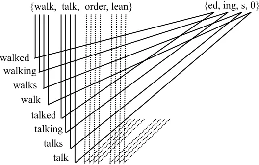
Unsupervised learning of morphology has been an important task because of the bene-fits it provides to many other natural language processing applications such as machine translation, information retrieval, question answering, and so forth. Morphological paradigms provide a natural way to capture the internal morphological structure of a group of morphologically related words. Following Goldsmith (2001) and Monson (2008), we use the termparadigmas consisting of a set of stems and a set of suffixes where each combination of a stem and a suffix leads to a valid word form, for example,

{walk,talk,order,yawn}{s,ed,ing}generating the surface formswalk+ed,walk+s,walk+ing, talk+ed,talk+s,talk+ing,order+s,order+ed,order+ing,yawn+ed,yawn+s,yawn+ing. A sam-ple paradigm is given in Figure 1.

Recently, we introduced a probabilistic hierarchical clustering model for learning hierarchical morphological paradigms (Can and Manandhar 2012). Each node in the hierarchical tree corresponds to a morphological paradigm and each leaf node consists of a word. A single tree is learned, where different branches on the hierarchical tree

Submission received: 29 June 2016; revised version received: 30 July 2017; accepted for publication: 1 March 2018.

{walk, talk, order, lean} {ed, ing, s, 0}

walked walking

walks walk

talked talking

talks talk

Figure 1

An example paradigm.

correspond to different morphological forms. Well-defined paradigms in the lower levels of trees were learned. However, merging of the paradigms at the upper levels led to undersegmentation in that model. This problem led us to search for ways to learn multiple trees. In our current approach, we learn a forest of paradigms spread over several hierarchical trees. Our evaluation on Morpho Challenge data sets provides better results when compared to the previous method (Can and Manandhar 2012). Our results are comparable to current state-of-the-art results while having the additional benefit of inferring the hierarchical structure of morphemes for which no comparable systems exist.

The article is organized as follows: Section 2 introduces the related work in the field. Section 3 describes the probabilistic hierarchical clustering model with its mathematical model definition and how it is applied for morphological segmentation; the same section explains the inference and the morphological segmentation. Section 4 presents the experimental setting and the obtained evaluation scores from each experiment, and Section 5 concludes and addresses the potential future work following the model presented in this article.

2. Related Work

There have been many unsupervised approaches to morphology learning that focus solely on segmentation (Creutz and Lagus 2005a, 2007; Snyder and Barzilay 2008; Poon, Cherry, and Toutanova 2009; Narasimhan, Barzilay, and Jaakkola 2015). Others, such as Monson et al. (2008), Can and Manandhar (2010), Chan (2006), and Dreyer and Eisner (2011), learn morphological paradigms that permit additional generalization.

A popular paradigmatic model is Linguistica (Goldsmith 2001), which uses the Minimum Description Length principle to minimize the description length of a corpus based on paradigm-like structures called signatures. A signature consists of a list of suffixes that are seen with a particular stem—for example,order-{ed, ing, s}denotes a signature for the stemorder.

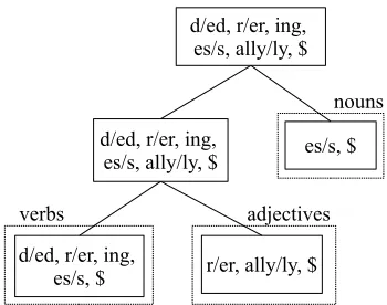
Figure 2

Examples of hierarchical morphological paradigms.

subsets of the lexicon, ranks them, and incrementally combines them in order to find the best segmentation of the lexicon. The proposed model addresses both inflectional and derivational morphology in a language independent framework. However, their model does not allow multiple suffixation (e.g., having multiple suffixes added to a single stem) whereas Linguistica allows this.

Monson et al. (2008) induce morphological paradigms in a deterministic framework named ParaMor. Their search algorithm begins with a set of candidate suffixes and collects candidate stems that attach to the suffixes (see Figure 2(b)). The algorithm gradually develops paradigms following search paths in a lattice-like structure. Proba-bilistic ParaMor, involving a statistical natural language tagger to mimic ParaMor, was introduced in Morpho Challenge 2009 (Kurimo et al. 2009). The system outperforms other unsupervised morphological segmentation systems that competed in Morpho Challenge 2009 (Kurimo et al. 2009) for the languages Finnish, Turkish, and German.

Can and Manandhar (2010) exploit syntactic categories to capture morphological paradigms. In a deterministic scheme, morphological paradigms are learned by pairing syntactic categories and identifying common suffixes between them. The paradigms compete to acquire more word pairs.

Chan (2006) describes a supervised procedure to find morphological paradigms within a hierarchical structure by applying latent Dirichlet allocation. Each paradigm is placed in a node on the tree (see Figure 2(a)). The results show that each paradigm corresponds to a part-of-speech such as adjective, noun, verb, or adverb. However, as the method is supervised, the true suffixes and segmentations are known in advance. Learning hierarchical paradigms helps not only in learning morphological segmenta-tion, but also in learning syntactic categories. This linguistic motivation led us toward learning the hierarchical organization of morphological paradigms.

Luo, Narasimhan, and Barzilay (2017) learn morphological families that share the same stem, such asfaithful,faithfully,unfaithful,faithless, and so on, that are all derived from faith. Those morphological families are learned as a graph and called

morpho-logical forests, which deviates from the meaning of the term forest we refer in this

article. Although learning morphological families has been studied as a graph learning problem in Luo, Narasimhan, and Barzilay (2017), in this work, we learn paradigms that generalize morphological families within a collection of hierarchical structures.

Narasimhan, Barzilay, and Jaakkola (2015) model the word formation with mor-phological chains in terms of parent-child relations. For example,playandplayfulhave a parent–child relationship as a result of adding the morphemefulat the end ofplay. These relations are modeled by using log-linear models in order to predict the parent relations. Semantic features as given by word2vec (Mikolov et al. 2013) are used in their model in addition to orthographic features for the prediction of parent–child relations. Narasimhan, Barzilay, and Jaakkola use contrastive estimation and generate corrupted examples as pseudo negative examples within their approach.

Our model is an extension of our previous hierarchical clustering algorithm (Can and Manandhar 2012). In that algorithm, a single tree is learned that corresponds to a hierarchical organization of morphological paradigms. The parent nodes merge the paradigms from the child nodes. But such merging of paradigms into a single structure causes unrelated paradigms to be merged resulting in lower segmentation accuracy. The current model addresses this issue by learning a forest of tree structures. Within each tree structure the parent nodes merge the paradigms from the child nodes. Multiple trees ensure that paradigms that should not be merged are kept separated. Additionally, in single tree hierarchical clustering, a manually defined context free grammar was employed to generate the segmentation of a word. In the current model, we predict the segmentation of a word without using any manually defined grammar rules.

3. Probabilistic Hierarchical Clustering

Chan (2006) showed that learning the hierarchy between morphological paradigms can help reveal latent relations in data. In the latent class model of Chan (2006), mor-phological paradigms in a tree structure can be linked to syntactic categories (i.e., part-of-speech tags). An example output of the model is given in Figure 2(a). Furthermore, tokens can be assigned to allomorphs or gender/conjugational variants in each paradigm.

Monson et al. (2008) showed that learning paradigms within a hierarchical model gives a strong performance on morphological segmentation. In their model, each paradigm is part of another paradigm, implemented within a lattice structure (see Figure 2(b)).

Motivated by these works, we aim to learn paradigms within a hierarchical tree structure. We propose a novel hierarchical clustering model that deviates from the current hierarchical clustering models in two aspects:

1. It is a generative model based on a hierarchical Dirichlet process (HDP) that simultaneously infers the hierarchical structure and morphological segmentation.

T_j T_k

a b c d

T_i

D_k={b, c, d} D_i={a, b, c, d}

D_j={b, c}

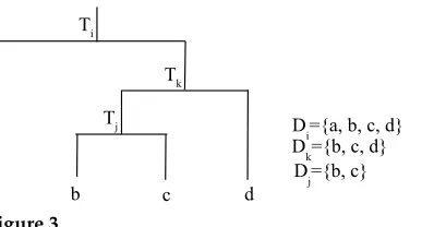
Figure 3

A portion of a tree rooted atiwith child nodesk,jwith corresponding data points they generate.

i,j,krefer to the tree nodes;Ti,Tj,Tkrefer to corresponding trees; andDi,Dj,Dkrefer to data

contained in trees.

Although not covered in this work, additional work can be aimed at discovering other types of latent information such as part-of-speech and allomorphs.

3.1 Model Overview

LetD = {x1,x2,. . .,xN}denote the input data where each xj is a word. Let Di⊆D

denote the subset of the data generated by tree rooted ati, then (see Figure 3):

D=D1∪D2∪ · · · ∪Dk (1)

whereDi = {x1i,x2i,. . .,x Ni i }.

The marginal probability of the data items in a given node in a treeiwith parameters θand hyperparametersβis given by:

p(Di)= Z

p(Di|θ)p(θ|β)dθ (2)

Given treeTithe data likelihood is given recursively by:

p(Di|Ti)= 





1

Zp(Di)p(Dl|Tl)p(Dr|Tr) ifiis an internal node with child nodes

landr, andZis the partition function p(Di) ifiis a leaf node

(3)

The term 1

Z(Di)p(Dl|Tl)p(Dr|Tr) corresponds to a product of experts model (Hinton

2002) comprising two competing hypotheses.1 _{Hypothesis H}

1 is given by p(Di) and

assigns all the data points in Di into a single cluster. Hypothesis H2 is given by

p(Dl|Tl)p(Dr|Tr) and recursively splits the data inDiinto two partitions (i.e., subtrees)

DlandDr. The factorZis the partition function or the normalizing constant given by:

Z= X

Di,Dl,Dr:Di=Dl∪Dr

p(Di)p(Dl|Tl)p(Dr|Tr) (4)

The recursive partitioning scheme we use is similar to that of Heller and Ghahramani (2005). The product of experts scheme used in this paper contrasts with the more conventional sum of experts mixture model of Heller and Ghahramani (2005) that would have resulted in the mixture π p(Di)+(1−π) p(Dl|Tl)p(Dr|Tr), where π

denotes the mixing proportion.

Finally, given the collection of treesT={T1,T2,. . .,Tn}, the total likelihood of data

in all trees is defined as follows:

p(D|T)= |T|

Y

i

p(Di|Ti) (5)

Trees are generated from a DP. Let T = {T1,T2,. . .,Tn} be a set of trees. Ti is

sampled from a DP as follows:

F∼DP(α,U) (6)

Ti ∼F (7)

whereαdenotes the concentration parameter of the DP.Uis a uniform base distribution that assigns equal probability to each tree. We integrate outF, which is a distribution over trees, instead of estimating it. Hence, the conditional probability of sampling an existing tree is computed as follows:

p(Tk|T,α,U)= _NN₊k_α (8)

whereNkdenotes the number of words inTkandNdenotes the total number of words

in the model. A new tree is generated with the following:

p(T|T|+1|T,α,U)=

α/k

N+α (9)

3.2 Modeling Morphology with Probabilistic Hierarchical Clustering

repairing

{order,yell,talk,repair,cook}{0,s,ed,ing}

{order}{0,ing}

order ordering

repairs {repair}{s,ing}

{yell,talk,repair,cook}{s,ed,ing}

{yell,talk,cook}{ed,ing}

{cook}{ed,ing}

yelling talking cooked cooking

slowly {quick,slow}{0,ly,ness}

{quick}{0,ly}

quick quickly

slow

{slow}{0,ly} {slow}{0,ly,ness}

slowness

Figure 4

A sample hierarchical tree structure that illustrates the clusters in each node (i.e., paradigms). Each node corresponds to a cluster (i.e., morphological paradigm) and the leaf nodes correspond to input data. The figure shows the ideal forest of trees that one expects given the input data.

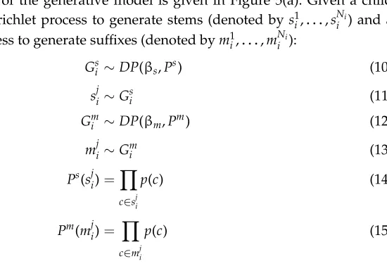
The plate diagram of the generative model is given in Figure 5(a). Given a child nodei, we define a Dirichlet process to generate stems (denoted bys1

i,. . .,s Ni i ) and a

separate Dirichlet process to generate suffixes (denoted bym1_i,. . .,mNi i ):

Gs_i ∼DP(β_s,Ps) (10)

sj_i∼Gs_i (11)

Gm_i ∼DP(β_m,Pm) (12)

mj_i∼Gm_i (13)

Ps(sj_i)=Y

c∈sj_i

p(c) (14)

Pm(mj_i)= Y

c∈mj_i

p(c) (15)

whereDP(β_s,Ps) is a Dirichlet process that generates stems,β_sdenotes the concentra-tion parameter, and Ps is the base distribution. Gs_i is a distribution over the stems sj_i in nodei. Correspondingly, DP(β_m,Pm) is a Dirichlet process that generates suffixes with analogous parameters. Gm_i is a distribution over the suffixes mj_i in node i. For smaller values of the concentration parameter, it is less likely to generate new types. Thus, sparse multinomials can be generated by the Dirichlet process yielding a skewed distribution. We setβ_s<1 andβ_m<1 in order to generate a small number of stem and suffix types.sj_iandmj_iare thejth stem and suffix instance in theith node, respectively.

The base distributions for stems and suffixes are given by Equation (14) and Equa-tion (15). Here,c denotes a single letter or character. We assume that letters are dis-tributed uniformly (Creutz and Lagus 2005b), wherep(c)=1/Afor an alphabet having Aletters. Our model will favor shorter morphemes because they have less factors in the joint probability given by Equations (14) and (15).

Figure 5

The DP model for the child nodes (on the left) illustrates the generation of wordstalking, cooked,

yelling. Each child node maintains its own DP that is independent of DPs from other nodes. The

HDP model for the root nodes (on the right) illustrates the generation of wordsyelling, talking,

repairs. In contrast to the DPs in the child nodes, in the HDP model, the stems/suffixes are shared across all root HDPs.

trees. The model will favor stems and suffixes that are already generated in one of the trees. The HDP for a root nodeiis defined as follows:

Fs_i ∼DP(β_s,Hs) (16)

Hs ∼DP(α_s,Ps) (17)

sj_i ∼Fs_i (18)

ψz_i ∼Hs (19)

Fm_i ∼DP(β_m,Hm) (20)

Hm ∼DP(α_m,Pm) (21)

mj_i ∼Fm_i (22)

φz_i ∼Hm (23)

where the base distributionsHs andHmare drawn from the global DPsDP(α_s,Ps) and DP(α_m,Pm). Here,ψ_izdenotes the stem typezin nodei, andφz_i denotes the suffix typez in nodei, which are drawn fromHsandHm(i.e., the global DPs), respectively. The plate

diagram of the HDP model is given in Figure 5(b).

order sleep pen book walk

s ing

0

Global Chinese restaurant

order sleep walk

ing s

D₁={walks,walking,ordering, sleeps,sleeping}

order walk

s 0

D₃={walk,order,orders} book walk

pen

s 0

D₂={pen,pens,book,books,walk}

ed …... ing

…... …...

….. _…...

….... Local Chinese restaurants

ly es ed …………....

………….... quick

Figure 6

A depiction of the Chinese restaurant franchise (i.e., global vs. local CRPs).

S1={walk,order,sleep,etc.},M1={s,ing},S2={pen,book},M2={0,s},S3={walk,order},

M3={0,s}, where 0 denotes an empty suffix. For each stem type in the distinct trees, a customer

is inserted in the global restaurant. For example, there are two stem customers that are being

served the stem typewalkbecausewalkexists in two different trees.

and for each stem/suffix type there exists only one table in each node (i.e., restaurant). Customers are the stem or suffix tokens. Whenever a new customer,sj_i ormj_i, enters a restaurant, if the table,ψz_i orφz_i, serving that dish already exists, the new customer sits at that table. Otherwise, a new table is generated in the restaurant. A change in one of the restaurants in the leaf nodes leads to the update in each restaurant all the way to the root node. If the dish is not available in the root node, a new table is created for that root node and a global customer is also added to the global restaurant. If no global table exists for that dish, a new global table serving the dish is also created. This can be seen as a Chinese restaurant franchise where each node is a restaurant itself (see Figure 6).

In order to calculate the joint likelihood of the model, we need to consider both trees and global stem/suffix sets (i.e., local and global restaurants). The model is exchange-able because it is a CRP—which means that the order the words are segmented does not alter the joint probability. The joint likelihood of the entire model for a given collection of treesT={T1,T2,. . .,Tn}is computed as follows:

p(D|T)= |T|

Y

i

p(Di|Ti) (24)

= |T|

Y

i

p(Si|Ti)p(Mi|Ti) (25)

=p(Sroot)p(Mroot)

|T|

Y

i=1

i6=root

wherep(Si|Ti) andp(Mi|Ti) are computed recursively:

p(Si|Ti)= ₁

Zp(Si)p(Sl|Tl)p(Sr|Tr) ifiis an internal node with child nodeslandr

p(Si) ifiis a leaf node

(27)

whereZis the normalization constant. The same also applies forMi.

Following the CRP, the joint probability of the stems in each root nodeTi,Srooti =

{s1

i,s2i,. . .,s Ni i }, is:

p(Sroot)=

|T|

Y

i

p(s1_i,s2_i,. . .,sNi

i ) (28)

= |T|

Y

i

p(s1_i)p(s2_i|s1_i). . .p(sNi

i |s1i,. . .,s Ni−1

i ) (29)

=





|T|

Y

i 



Γ(β_s) Γ(Ni+βs)

βLsi−1 s

Ls i Y

j=1

(ns_ij−1)!



 

 (30)





Γ(α_s) Γ(P

sj∈Ksk s j +αs)

αK_ss−1

Ks Y

j=1

(ks_j −1)!Ps(sj) 



where the first line in Equation (30) corresponds to the stem CRPs in the root nodes of the trees (see Equation (2.22) in Can [2011] and Equation (A.1) in Appendix A). The second line in Equation (30) corresponds to the global CRP of stems. The second factor in the first line of Equation (30) corresponds to the case whereLs

i stem types are generated

the first time, and the third factor in the first line corresponds to the case, where for each of theLs

i stem types at nodei, there arensijstem tokens of typej. The first factor accounts

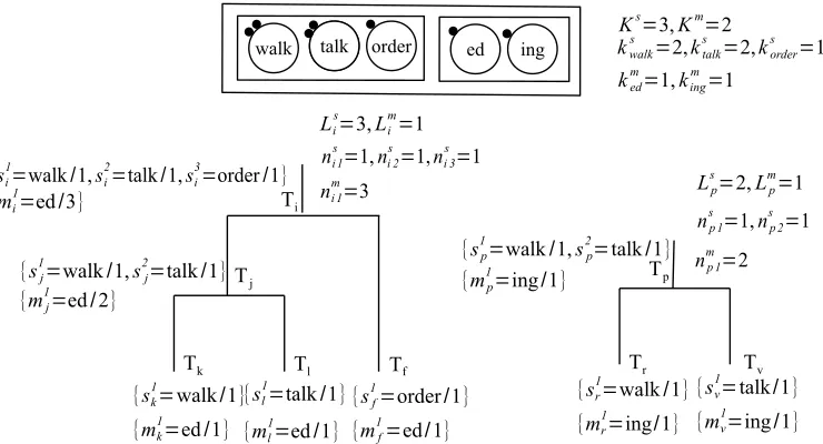
for all denominators from both cases. Similarly, the second and the fourth factor in the second line of Equation (30) corresponds to the case whereKsstem types are generated globally (i.e., stem tables in the global restaurant), the third factor corresponds to the case where, for each of theKs stem types, there areks_j stems of typejin distinct trees. A sample hierarchical structure is given in Figure 7.

The joint probability of stems in a child nodeTi,Si={s1i,s2i,. . .,s Ni

i }, which belong

to stem tables{ψ1_i,ψ2_i,. . .}that index the items on the global menu is reduced to:

p(Si)=

Γ(β_s) Γ(Ni+βs)

βLsi−1 s

Ls i Y

j=1

(ns_ij−1)!Ps(ψj_i) (31)

order

talk _{ed ing}

walk

Li s

=3,Li m

=1

ni 1 s

=1,ni 2 s

=1,ni 3

s

=1

ni 1 m

=3

{si

1

=walk/1,si

2

=talk/1,si

3

=order/1}

{mi

1

=ed/3}

{sj

1

=walk/1,sj

2

=talk/1}

{mj

1

=ed/2}

{sk

1

=walk/1}

{mk

1

=ed/1}

{sl

1

=talk/1}

{ml

1

=ed/1}

{sf

1

=order/1}

{mf

1

=ed/1}

{sp

1

=walk/1,sp

2

=talk/1}

{mp

1

=ing/1}

{sr

1

=walk/1}

{mr

1

=ing/1}

{sv

1

=talk/1}

{mv

1

=ing/1}

Ks

=3,Km

=2

kwalk s

=2,ktalk

s

=2,korder s

=1

ked m

=1,king

m

=1

Lp s₌

2,Lp m₌

1 np 1

s

=1,np 2

s

=1

np 1 m

=2

Ti

Tj

Tk Tl Tf

Tp

Tr Tv

Figure 7

A sample hierarchical structure that containsD={walk+ed,talk+ed,order+ed,walk+ing,

talk+ing}and the corresponding global tables. Heres1

k=walk/1 denotes the first stemwalkin

nodekwith frequency 1.

(i.e., customersj_isitting at tableψz_i) is computed as follows (see Teh 2010 and Teh et al. 2006):

p(sj_i=z|Si−s j i_,β

s,Ps) =                   

n−s j i iz

Ni−1+βs if

ψz_i ∈Ψi

β_sPs(sj_i)

Ni−1+βs otherwise (for an internal node)

β_sHs_(ψz i|αs,Ps)

Ni−1+βs otherwise (for a root node)

(32)

whereΨ_idenotes the table indicators in nodei,n−s j i

iz denotes the number of stem tokens

that belong to typezin nodeiwhen the last instancesj_iis excluded.

If the stem (customer) does not exist in the root node (i.e., chooses a non-existing dish type in the root node), the new stem’s probability is calculated as follows:

Hs(ψz_i|α_s,Ps) =

        

ks_z P

sj∈Ksk s

j+αs ifj

∈Ks

α_sPs(sz) P

sj∈Ksk s j+αs

otherwise

(33)

Analogously to Equations (30)–(33) that apply to stems, the corresponding equa-tions for suffixes are given by Equaequa-tions (34)–(37).

p(Mroot)= 



|T|

Y

i 



Γ(β_m) Γ(Ni+βm)

βLmi−1 m

Lm i Y

j=1

(nm_ij −1)!



 

 (34)





Γ(α_m) Γ(P

mj∈Kmk m

j +αm)

αK_mm−1

Km Y

j=1

(km_j −1)!Pm(mj) 



p(Mi)=

Γ(β_m) Γ(Ni+βm)

βLmi−1 m

Lm i Y

j=1

(nm_ij −1)!Pm(φj_i) (35)

p(mj_i=z|Mi−m j

i_,βm,Pm_{) =} 

        

        

n−m j i iz

Ni−1+βm if

φz_i ∈Φ_i

β_mPm_(mj i)

Ni−1+βm otherwise (for an internal node)

β_mHm(φz_i|α_m,Pm)

Ni−1+βm otherwise (for a root node)

(36)

Hm(φz_i|α_m,Pm) =



   

   

kmz P

mj∈Kmk m

j +αm ifj

∈Km

α_mPm(mz) P

mj∈Kmk m

j +αm otherwise

(37)

whereMi={m1i,m1i,. . .,m Ni

i }is the set of suffixes in nodeibelonging to global suffix

types{φ1_i,φ2_i,. . .};Nm_i is the number of local suffix types;nm_ij is the number of suffix tokens of typejin nodei;Kmis the total number of suffix types; andkm_j is the number of trees that contain suffixes of typej.

3.3 Metropolis-Hastings Sampling for Inferring Trees

Trees are learned along with the segmentations of words via inference. Learning trees involves two steps: 1) constructing initial trees; 2) Metropolis-Hastings sampling for inferring trees.

3.3.1 Constructing Initial Trees.Initially, all words are split at random points with uniform probability. We use an approximation to construct the intial trees. Instead of computing the full likelihood of the model, for each tree, we only compute the likelihood of a single DP and assume that all words belong to this DP. The conditional probability of inserting wordwj=s+min treeTkis given by:

p(Tk,wj=s+m|D,T,α,βs,βm,Ps,Pm,U)

=p(Tk|T,α,U)p(wj=s+m|Dk)

We use Equation (8) and (9) for computing the conditional probabilityp(Tk|T,α,U) of

choosing a particular tree. Once a tree is chosen, a branch to insert is selected at random. The algorithm for constructing the initial trees is given in Algorithm 1.

3.3.2 Metropolis-Hastings Sampling. Once the initial trees are constructed, the hierar-chical structures yielding a global maximum likelihood are inferred by using the Metropolis Hastings algorithm (Hastings 1970). The inference is performed by itera-tively removing a word from a leaf node from a tree and subsequently sampling a new tree, a position within the tree, and a new segmentation (see Algorithm 2). Trees are sampled with the conditional probability given in Equations (8) and (9). Hence, trees with more words attract more words, and new trees are created proportional to the hyperparameterα.

Once a tree is sampled, we draw a new position and a new segmentation. The word is inserted at the sampled position with the sampled segmentation. The new model is either accepted or rejected with the Metropolis-Hastings accept-reject criteria. We also use a simulated annealing cooling schedule by assigning an initial temperatureγto the system and decreasing the temperature at each iteration. The accept probability we use is given by:

PAcc=

pnext(D|T)

pcur(D|T) γ1

(39)

where pnext(D|T) denotes the likelihood of the data under the altered model and

pcur(D|T) denotes the likelihood of data under the current model before sampling. The

normalization constant cancels out because it is the same for the numerator and the denominator. Ifpnext(D|T)

1

γ _>p

cur(D|T) 1

γ_{, then the new sample is accepted: otherwise,}

Algorithm 1Construction of the initial trees.

1: input:dataD:={w1 _=s1_+m1_{,. . .,w}N_=sN_+mN_}

2: initialize:The trees in the model:T:=∅

3: Forj=1. . .N

4: Choosewjfrom the corpus.

5: Sample,Tkas a new empty tree or existing tree fromT, and, a split pointwj=s+m

from the joint distribution (see Equation 38): p(Tk,wj=s+m|D,T,α,βs,βm,Ps,Pm,U)

6: ifTk∈T then

7: Draw a nodesfromTkwith uniform probability

8: AssignTkas a sibling ofTs: Ts :=Ts+Tk(i.e.,Ts is new tree withTkand oldTs

as children) 9: else

10: Tkis an empty tree. AddTkintoT: T:=T∪Tk

11: Dk:={wj=s+m}(i.e., wordwj=s+mis assigned intoTk)

12: end if

13: Removewjfrom the corpus

14: End For

Algorithm 2Learning the trees with Metropolis-Hastings algorithm

1: input:dataD:={w1 =s1+m1,. . .,wN =sN+mN}, initial treesT, initial

temperatureγ, the target temperatureκ, temperature decrementη

2: initialize:pcur(D|T) :=p(D|T)

3: whileγ > κdo

4: Choose the leaf nodejfromalltrees with uniform probability 5: LetDj:={wj=sold+mold}

6: Draw a split pointwj_=snew_+mnew_{with uniform probability}

7: Draw a treeTkwith probabilityp(Tk|T,α,U) (see Equations 8 and 9)

8: ifTk∈Tthen

9: Draw a sibling nodesfromTkwith uniform probability

10: Ts:=Ts+Tk(see Figure 8)

11: else

12: Create a new treeTk

13: T:=T∪Tk

14: Dk:={wj=snew+mnew}

15: end if

16: rand∼Normal(0, 1)

17: pnext:=p(D|T) (see Equation 24)

18: ifpnext(D|T)>=pcur(D|T)orrand< _p

next(D|T) pcur(D|T)

γ1

then

19: Accept the new tree structure 20: pcur(D|T) := pnext(D|T)

21: end if

22: γ:=γ−η

23: end while

24: output: T

the new model is still accepted with a probability pAcc. The system is cooled in each

iteration with decrementsη. We refer to Section 4 for details of parameter settings.

γ←γ−η (40)

3.4 Morphological Segmentation

Once the model is learned, it can be used for the segmentation of novel words. We use only root nodes for the segmentation. Viterbi decoding is used in order to find the morphological segmentation of each word having the maximum probability:

arg max

s1_,···,sa_,m1_,...,mbp(w

k_=s1_{,· · ·,s}a_,m1_{,· · ·,m}b_|D,α

s,βs,Hs,Ps,αm,βm,Hm,Pm)

=

a Y

j=1 |T|

X

i=1

i=root

p(sj_i|Si,αs,βs,Hs,Ps)

b Y

j=1 |T|

X

i=1

i=root

p(mj_i|Mi,αm,βm,Hm,Pm)

(41)

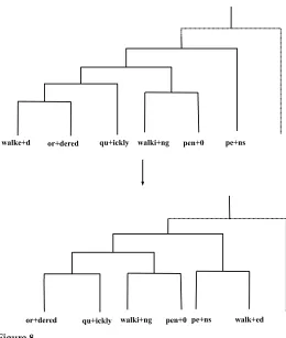
walke+d or+dered qu+ickly walki+ng pen+0 pe+ns

or+dered qu+ickly walki+ng pen+0 pe+ns walk+ed

Figure 8

A sampling step in Metropolis-Hastings algorithm.

3.5 Example Paradigms

A sample of root paradigms learned by our model for English is given in Table 1. The model can find similar word forms (i.e., separat+ists, medal+ists, hygien+ists) that are grouped in the neighbor branches in the tree structure (see Figures 9, B.1, and B.2 for sample paradigms learned in English, Turkish, and German).

Paradigms are captured based on the similarity of either stems or suffixes. Having the same stem such as co-chair (co-chairman, co-chairmen) or trades (trades+man, trades+men) allows us to find segmentations such as co-chair+man vs. co-chair+men and trades+man vs. trades+men. Although we assume a stem+suffix segmentation, other types of segmentation, such as prefix+stem, are also covered. However, stem alterations and infixation are not covered in our model.

4. Evaluation

Table 1

Example paradigms in English.

{final, ungod, frequent, pensive} {ly}

{kind, kind, kind} {est, er, 0}

{underrepresent, modul} {ation}

{plebe, hawai, muslim-croat} {ian}

{compuls, shredd, compuls, shredd, compuls} {ion, er, ively, ers, ory}

{zion, modern, modern, dynam} {ism, ists}

{reclaim, chas, pleas, fell} {ing}

{mov, engrav, stray, engrav, fantasiz, reischau,

decilit, suspect} {ing, er, e}

{measur, measur, incontest, transport, unplay, reput}

{e, able}

{housewar, decorat, entitl, cuss, decorat, entitl, materi, toss, flay, unconfirm

linse, equipp} {es, ing, alise, ed}

{fair, norw, soon, smooth, narrow, sadd, steep, noisi, statesw, narrow}

{est, ing}

{rest, wit, name, top, odor, bay, odor, sleep} {less, s}

{umpir, absorb, regard, embellish, freez, gnash} {ing}

{nutrition, manicur, separat, medal, hygien, nutrition, genetic, preservation}

{0, ists}

information. In other words, we use only the word types (not tokens) in training. We do not address the ambiguity of words in this work and leave this as future research.

In all experiments, the initial temperature of the system is set γ=2 and it is reduced toγ=0.01 with decrements η=0.0001 (see Equation (39)). Figure 10 shows the time required for the log likelihoods of the trees of sizes 10K, 16K, and 22K to converge. We fixedα_s=α_m =β_s=β_m =0.01 and α=0.0005 in all our experiments. The hyperparameters are set manually as a result of several experiments. These are the optimum values obtained from a number of experiments.2

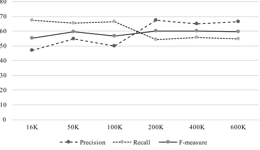
Precision, recall, and F-score values against training set sizes are given in Figures 11 and 12 for English and Turkish, respectively.

4.1 Morpho Challenge Evaluation

Although we experimented with different sizes of training sets, we used a randomly chosen 600K words from the English and 200K words from the Turkish and German data sets for evaluation purposes.

Evaluation is performed according to the method proposed in Morpho Challenge (Kurimo et al. 2010a), which in turn is based on evaluation used by Creutz and Lagus (2007). The gold standard evaluation data set utilized within the Morpho Challenge is a hidden set that isnotavailable publicly. This makes the Morpho Challenge evaluation different from other evaluations that provide test data. In this evaluation, word pairs

sl ay + er ta xp ay + er br ic kl ay + er po li cy -m ak + er gr an t-m ak + in g ca nn + in g pl ay -a ct + in g di sh was h+ in g un fe el + in g co m m ut + in g lig ht -e m it t+ in g bu ry + in g en er gy -p ro du c+ in g do er + in g co m pr is + in g un cl ot h+ ed ci rc l+ ed un co nv er t+ ed te le co m m ut + in g ta ba n+ la rı nı zı n ac ı+ la rı nı zı n sa tı cı + la rl a uz an tı + la rl a ot ur um + la rı n sa tı cı + la rı n uy ar ıc ı+ la ra sa va şç ı+ la ra sa va şç ı+ ya eş ya la r+ ın ı şa n+ ın ı na m + ın ı te m as + ın ı ad ım + ın ı ek ip m an + ın ı ad ım + ın sc hw er + m ac he n sc hw er + kr an k w et t+ m ac he n w et t+ kr im in al it ae t w oc he n+ lo hn au sl ae nd er + kr im in al it ae t w oc he n+ ze it sc hr if t pl ay + st at io n ra da r+ w ag en ra da r+ sy st em e ra da r+ st at io n sk i+ st at io n Figure 9

Sample hierarchies in English, Turkish, and German.

sharing at least one common morpheme are sampled. For precision, word pairs are sampled from the system results and checked against the gold standard segmentations. For recall, word pairs are sampled from the gold standard and checked against the system results. For each matching morpheme, 1 point is given. Precision and recall are calculated by normalizing the total obtained scores.

–1.60E+07 –1.50E+07 –1.40E+07 –1.30E+07 –1.20E+07 –1.10E+07 –1.00E+07 –9.00E+06 –8.00E+06 –7.00E+06 –6.00E+06

1 ₆₃

12

5

18

7

24

9

31

1

37

3

43

5

49

7

55

9

62

1

68

3

74

5

80

7

86

9

93

1

99

3

105

5

111

7

11

79

124

1

130

3

136

5

142

7

148

9

155

1

161

3

167

5

M

ar

gi

n

al

li

k

el

ih

oo

d

Time (min.)

16K 22K Figure 10

The likelihood convergence in time (in minutes) for data sets of size 16K and 22K.

0 10 20 30 40 50 60 70 80

16K 50K 100K 200K 400K 600K

Precision Recall F-measure

Figure 11

English results for different size of data.

English results are given in Table 2. For English, the Base Inference algorithm of Lignos (2010) obtained the highest F-measure in Morpho Challenge 2010 among other competing unsupervised systems. Our model is ranked fourth among all unsupervised systems with a F-measure 60.27%.

German results are given in Table 3. Our model outperforms other unsupervised models in Morpho Challenge 2010 with a F-measure 50.71%.

Turkish results are given in Table 4. Again, our model outperforms other unsuper-vised participants, achieving a F-measure 56.41%.

0 10 20 30 40 50 60 70 80

16K 50K 100K 200K 400K 600K

Precision Recall F-measure

Figure 12

Turkish results for different size of data.

Table 2

Morpho Challenge 2010 experimental results for English.

System Precision (%) Recall (%) F-measure (%)

Hierarchical Morphological Segmentation 55.60 65.80 60.27

Single Tree Prob. Clustering (Can and Manandhar 2012)

55.60 57.58 57.33

Base Inference (Lignos 2010) 80.77 53.76 64.55

Iterative Compounding (Lignos 2010) 80.27 52.76 63.67

Aggressive Compounding (Lignos 2010) 71.45 52.31 60.40

Nicolas (Nicolas, Farr´e, and Molinero 2010) 67.83 53.43 59.78

Morfessor Baseline (Creutz and Lagus 2002) 81.39 41.70 55.14

Morpho Chain (Narasimhan, Barzilay, and Jaakkola 2015)

74.87 39.01 50.42

Morfessor CatMAP (Creutz and Lagus 2005a) 86.84 30.03 44.63

Table 3

Morpho Challenge 2010 experimental results for German.

System Precision (%) Recall (%) F-measure (%)

Hierarchical Morphological Segmentation 47.92 53.84 50.71

Single Tree Prob. Clustering (Can and Manandhar 2012)

57.79 32.42 41.54

Base Inference (Lignos 2010) 66.38 35.36 46.14

Iterative Compounding (Lignos 2010) 62.13 34.70 44.53

Aggressive Compounding (Lignos 2010) 59.41 37.21 45.76

Morfessor Baseline (Creutz and Lagus 2002) 82.80 19.77 31.92

Morfessor CatMAP (Creutz and Lagus 2005a) 72.70 35.43 47.64

Table 4

Morpho Challenge 2010 experimental results for Turkish.

System Precision (%) Recall (%) F-measure (%)

Hierarchical Morphological Segmentation 57.70 55.18 56.41

Single Tree Prob. Clustering (Can and Manandhar 2012)

72.36 25.81 38.04

Base Inference (Lignos 2010) 72.81 16.11 26.38

Iterative Compounding (Lignos 2010) 68.69 21.44 32.68

Aggressive Compounding (Lignos 2010) 55.51 34.36 42.45

Nicolas (Nicolas, Farr´e, and Molinero 2010) 79.02 19.78 31.64

Morfessor Baseline (Creutz and Lagus 2002) 89.68 17.78 29.67

Morpho Chain (Narasimhan, Barzilay, and Jaakkola 2015)

69.25 31.51 43.32

Morfessor CatMAP (Creutz and Lagus 2005a) 79.38 31.88 45.49

Table 5

Comparison with Single Tree Probabilistic Clustering for English.

System Precision (%) Recall (%) F-measure (%)

Hierarchical Morphological Segmentation 67.75 53.93 60.06

Single Tree Prob. Clustering (Can and Manandhar 2012)

55.60 57.58 57.33

Table 6

Comparison with Single Tree Probabilistic Clustering for German.

System Precision (%) Recall (%) F-measure (%)

Hierarchical Morphological Segmentation 33.93 65.31 44.66

Single Tree Prob. Clustering (Can and Manandhar 2012)

57.79 32.42 41.54

Table 7

Comparison with Single Tree Probabilistic Clustering for Turkish.

System Precision (%) Recall (%) F-measure (%)

Hierarchical Morphological Segmentation 64.39 42.99 51.56

Single Tree Prob. Clustering (Can and Manandhar 2012)

72.36 25.81 38.04

4.2 Additional Evaluation

Table 8

Comparison with Morpho Chain model for English based on Morpho Chain evaluation.

System Precision (%) Recall (%) F-measure (%)

Hierarchical Morphological Segmentation 67.41 62.5 64.86

Morpho Chain 72.63 78.72 75.55

Table 9

Comparison with Morpho Chain model for Turkish based on Morpho Chain evaluation.

System Precision (%) Recall (%) F-measure (%)

Hierarchical Morphological Segmentation 89.30 48.22 62.63

Morpho Chain 70.49 63.27 66.66

calculated based on these matching segmentation points. In addition, this evaluation does not use the hidden gold data sets. Instead, the test sets are created by aggregating the test data from Morpho Challenge 2005 and Morpho Challenge 2010 (as reported in Narasimhan, Barzilay, and Jaakkola [2015]) that provide segmentation points.3

We used the same trained models as in our Morpho Challenge evaluation. The English test set contains 2,218 words and the Turkish test set contains 2,534 words.4

The English results are given in Table 8 and Turkish results are given in Table 9. For all systems, Morpho Chain evaluation scores are comparably higher than the Morpho Challenge scores. There are several reasons for this. In the Morpho Challenge evaluation, the morpheme labels are considered rather than the surface forms of the morphemes. For example,pantolon+u+yla[with his trousers] andemel+ler+i+yle[with his desires] have got both possessive morpheme (uandi) that is labeled withPOSand relational morpheme (ylaandyle) labeled withRELin common. This increases the total number of points that is computed over all word pairs, and therefore lowers the scores. Secondly, in the Morpho Chain evaluation, only the gold segmentation that has the maximum match with the result segmentation is chosen for each word (e.g.,yazımıza has two gold segmentations: yaz+ı+mız+a [to our summer] and yazı+mız+a; [to our writing]). In contrast, in the Morpho Challenge evaluation all segmentations in the gold segmentation are evaluated. This is another factor that increases the scores in Morpho Chain evaluation. Thus, the Morpho Chain evaluation favors precision over recall. Indeed, in the Morpho Challenge evaluation, the Morpho Chain system has high precision but their model suffers from low recall due to undersegmentation (see Tables 2 and 4).

It should be noted that the output of our system is not only the segmentation points, but also the hierarchical organization of morphological paradigms that we believe is novel in this work. However, because of the difficulty in measuring the quality of hier-archical paradigms, which will require a corresponding hierhier-archically organized gold data set, we are unable to provide an objective measure of the quality of hierarchical

3 In addition to the hidden test data, Morpho Challenge also provides separate publicly available test data. 4 Because of the unavailability of word2vec word embeddings for German, we were unable to perform

structures learned. We present different portions from the obtained trees in Appendix B (see Figures B.1 and B.2).5It can be seen that words sharing the same suffixes are gath-ered closer to each other, such asreestablish+ed,reclassifi+ed,circl+ed,uncloth+ed, and so forth. Secondly, related morphological families gather closer to each other, such as impress+ively,impress+ionist,impress+ions,impress+ion.

5. Conclusions and Future Work

In this article, we introduce a tree structured Dirichlet process model for hierarchical morphological segmentation. The method is different compared with existing hierar-chical and non-hierarhierar-chical methods for learning paradigms. Our model learns mor-phological paradigms that are clustered hierarchically within a forest of trees.

Although our goal in this work is on hierarchical learning, our model shows com-petitive performance against other unsupervised morphological segmentation systems that are designed primarily for segmentation only. The system outperforms other un-supervised systems in Morpho Challenge 2010 for German and Turkish. It also out-performs the more recent Morpho Chain (Narasimhan, Barzilay, and Jaakkola 2015) system on the Morpho Challenge evaluation for German and Turkish.

The sample paradigms learned show that these can be linked to other types of latent information, such as part-of-speech tags. Combining morphology and syntax as a joint learning problem within the same model can be a fruitful direction for future work.

The hierarchical structure is beneficial because we can have both compact and more general paradigms at the same time. In this article, we use the paradigms only for the segmentation task, and applications of hierarchy learned is left as future work.

Appendix A. Derivation of the Full Joint Distribution

LetD = {s1_,s2_{,. . .,s}N_{}denote the input data where eachs}j_{is a data item. A particular}

setting of a table withNcustomers has a joint probability of:

p(s1,. . .,sN|α,P)=p(s1|α,P)p(s2|s1,α,P)p(s3|s1,s2,α,P). . .p(sN|s1,. . .,sN−1,α,P)

= αL

α(1+α)(2+α)(N−1+α)

L Y

i=1

P(si)

L Y

i=1

(n_si −1)!

= Γ(α) Γ(N+α)α

L−1

L Y

i=1

(n_si−1)! L Y

i=1

P(si) (A.1)

For each customer, either a new table is created or the customer sits at an occupied table. For each table, at least one table creation is performed, which forms the second and the fourth factor in the last equation. Once the table is created, factors that represent the number of customers sitting at each table are chosen accordingly, which refers to the third factor in the last equation. All factors withαare aggregated in the first factor in terms of a Gamma function in the last equation.

Appendix B. Sample Tree Structures ba ch + m an tr ad es + m en tr ad es + m an co -c ha ir + m an ba ch + m an ro ff + m an tu ch + m en co -c ha ir co -c ha ir + m en jo ur ne y+ s' jo ur ne y+ m an se le ct + m en jo ur ne y+ m en en gl is h+ m en su m m er + li ke su m m er + ti m e be st + dr es se d w or st + dr es se d be st + qu al if ie d su m m er + fe st cl an s+ m an cl an s+ m en st ee d+ m an br ee d+ er br ee d+ in g br ee d+ en 's po un d+ s po un d+ ag e po un d+ er fa z+ ed fr ac tu r+ ed un in vo lv + ed re es ta bl is h+ ed un sa nc ti on + ed un sh ap + ed re cl as si fi + ed un ta le nt + ed co nk + ed ci rc l+ ed un cl ot h+ ed un co nv er t+ ed pa rt it io n+ ed lig ht -e m it t+ in g bu ry + in g en er gy -p rd uc + in g di sq ui et + in g se lf -p ro pe ll + ed do er + in g co m ri s+ in g dr ug -s ni ff + in g un ex ci t+ in g w al k+ in g oi l-dr il l+ in g un di vi de + d cu e+ d Figure B.1

di pl om a+ la rı nd a kı rı k+ la rı nd a ar aş tı rm a+ la rı dı r bu n+ la rd ır ko m ut an + ıd ır te m in at + ıd ır m ak in a+ la r sa vc ı+ la rd an m ak in a+ la rd ır sı ğı r+ la rd an or m an + la rd a sı ca kl ık + ta te m in at + la te m in at + tı r po li go n+ la rı nı n fı rt ın a+ la rd an pa tl am a+ la rd an so ru m lu lu k+ la rl a pa tl am a+ la rı nı n fı rt ın a+ la rı nı n po li go n+ la rı nd a so ru m lu lu k+ la rı nı al ış ka nl ık + la rd ır im ti ha n+ la rd a al ış ka nl ık + la r im ti ha n+ la rı nı so ru m lu lu k+ la rd an kı rı k+ kı rı k+ la rı nı n kı rı k+ la rd a te m in at + ın te m in at + a sa vc ı+ nı n sa vc ı+ la rı nı n ya ra la n+ dı ta sa rl a+ dı ya ra la n+ dı ğı ya ra la n+ m ış la rd ır ya ra la n+ ab il m ek tu t+ ab il m ek at an + ır la r ko ş+ m uş tu t+ m uş an la t+ am ad ım uy uy + am ad ım uy uy + am am ho şl an + an la r ku rt ar + ab il m ek çı k+ ab il m ek çı k+ am ad ım ku rt ar + ır la r çı kk ar + ır la r ku rt ar + ır la r du y+ am ad ım ku rt ar + am ad ım ka rş ıl aş ıl + m ad ı du r+ m uş du r+ ur du uy uy + an la r du r+ an la r ku tl ay + an la r ol uş tu r+ al ım tu t+ ac ağ ın ız ta k+ al ım ku tl ay + al ım bu lu nd ur + ac ağ ın ız so ru l+ ur ol uş tu r+ an la r so ru l+ sa yd ı so ru l+ m uş so ru l+ m ay a ya z+ an la r Figure B.2

Sample hierarchies in Turkish.

Acknowledgments

This research was supported by TUBITAK (The Scientific and Technological Research Council of Turkey) grant number 115E464. We thank Karthik Narasimhan for providing their data sets and code. We are grateful to Sami Virpioja for the evaluation of our results on the hidden gold data provided by Morpho Challenge. We thank our reviewers for critical feedback and spotting an error in our previous version of the article. Their comments have immensely helped improve the article.

References

Can, Burcu. 2011. Statistical Models for Unsupervised Learning of Morphology and POS tagging. Ph.D. thesis, Department of

Computer Science, The University of York.

Can, Burcu and Suresh Manandhar. 2010. Clustering morphological paradigms

using syntactic categories. InMultilingual

Information Access Evaluation I. Text Retrieval Experiments: 10th Workshop of the Cross-Language Evaluation Forum, CLEF 2009, Corfu, Greece, September 30 -October 2, 2009, Revised Selected Papers, pages 641–648, Corfu.

Can, Burcu and Suresh Manandhar. 2012. Probabilistic hierarchical clustering of

morphological paradigms. InProceedings of

the 13th Conference of the European Chapter of the Association for Computational Linguistics, EACL ’12, pages 654–663, Avignon. Chan, Erwin. 2006. Learning probabilistic

paradigms for morphology in a latent

Meeting of the ACL Special Interest Group on Computational Phonology and Morphology, SIGPHON ’06, pages 69–78, New York, NY.

Creutz, Mathias and Krista Lagus. 2002. Unsupervised discovery of morphemes. InProceedings of the ACL-02 Workshop on Morphological and Phonological Learning -Volume 6, MPL ’02, pages 21–30, Philadelphia, PA.

Creutz, Mathias and Krista Lagus. 2005a. Inducing the morphological lexicon of a natural language from unannotated text. InProceedings of the International and Interdisciplinary Conference on Adaptive Knowledge Representation and Reasoning (AKRR 2005), pages 106–113, Espoo. Creutz, Mathias and Krista Lagus. 2005b.

Unsupervised morpheme segmentation and morphology induction from text corpora using Morfessor 1.0. Technical Report A81. Helsinki University of Technology.

Creutz, Mathias and Krista Lagus. 2007. Unsupervised models for morpheme segmentation and morphology learning. ACM Transactions Speech Language Processing, 43:1–3:34.

Dreyer, Markus and Jason Eisner. 2011. Discovering morphological paradigms from plain text using a Dirichlet Process

mixture model. InProceedings of the 2011

Conference on Empirical Methods in Natural Language Processing, pages 616–627, Edinburgh.

Goldsmith, John. 2001. Unsupervised learning of the morphology of a natural

language.Computational Linguistics,

27(2):153–198.

Hastings, W. K. 1970. Monte Carlo sampling methods using Markov chains and their

applications.Biometrika, 57:97–109.

Heller, Katherine A. and Zoubin

Ghahramani. 2005. Bayesian hierarchical

clustering. InProceedings of the 22nd

International Conference on Machine Learning, ICML ’05, pages 297–304, Bonn.

Hinton, Geoff. 2002. Training products of experts by minimizing contrastive

divergence.Neural Computation,

14(8):1771–1800.

Kurimo, Mikko, Sami Virpioja, Ville

Turunen, and Krista Lagus. 2010a. Morpho Challenge Competition 2005–2010:

Evaluations and results. InProceedings of

the 11th Meeting of the ACL Special Interest Group on Computational Morphology and Phonology, SIGMORPHON ’10, pages 87–95, Uppsala.

Kurimo, Mikko, Sami Virpioja, Ville T. Turunen, Graeme W. Blackwood, and William Byrne. 2009. Overview and results

of Morpho Challenge 2009. InProceedings

of the 10th Cross-Language Evaluation Forum Conference on Multilingual Information Access Evaluation: Text Retrieval Experiments, CLEF’09, pages 578–597, Corfu. Kurimo, Mikko, Sami Virpioja, Ville T.

Turunen, Bruno G ´olenia, Sebastian Spiegler, Oliver Ray, Peter Flach, Oskar Kohonen, Laura Lepp¨anen, Krista Lagus, Constantine Lignos, Lionel Nicolas, Jacques Farr´e, and Miguel Molinero. 2010b. Proceedings of the Morpho Challenge 2010 Workshop. Technical Report TKK-ICS-R37. Aalto University. Lignos, Constantine. 2010. Learning from

unseen data. InProceedings of the Morpho

Challenge 2010 Workshop, pages 35–38, Espoo.

Luo, Jiaming, Karthik Narasimhan, and Regina Barzilay. 2017. Unsupervised learning of morphological forests. Transactions of the Association of Computational Linguistics, 5:353–364. Mikolov, Tomas, Kai Chen, Greg Corrado,

and Jeffrey Dean. 2013. Efficient estimation of word representations in vector space.

CoRR, abs/1301.3781.

Monson, Christian. 2008.Paramor: From

Paradigm Structure to Natural Language Morphology Induction. Ph.D. thesis, Language Technologies Institute, School of Computer Science, Carnegie Mellon University.

Monson, Christian, Jaime Carbonell, Alon Lavie, and Lori Levin. 2008. Paramor: Finding paradigms across morphology. InLecture Notes in Computer Science -Advances in Multilingual and Multimodal Information Retrieval; Cross-Language Evaluation Forum, CLEF 2007, pages 900–907, Springer, Berlin.

Narasimhan, Karthik, Regina Barzilay, and Tommi S. Jaakkola. 2015. An unsupervised method for uncovering morphological

chains.Transactions of the Association for

Computational Linguistics, 3:157–167. Nicolas, Lionel, Jacques Farr´e, and Miguel A.

Molinero. 2010. Unsupervised learning of concatenative morphology based on frequency-related form occurrence. In Proceedings of the Morpho Challenge 2010 Workshop, pages 39–43, Espoo.

Poon, Hoifung, Colin Cherry, and Kristina Toutanova. 2009. Unsupervised morphological segmentation with

log-linear models. InProceedings of Human

Conference of the North American

Chapter of the Association for Computational Linguistics, NAACL ’09, pages 209–217, Boulder, CO.

Snover, Matthew G., Gaja E. Jarosz, and Michael R. Brent. 2002. Unsupervised learning of morphology using a novel directed search algorithm: Taking the first

step. InProceedings of the ACL-02 Workshop

on Morphological and Phonological Learning, pages 11–20, Philadelphia, PA.

Snyder, Benjamin and Regina Barzilay. 2008. Unsupervised multilingual learning for morphological segmentation. In

Proceedings of ACL-08: HLT, pages 737–745, Columbus, OH.

Teh, Y. W. 2010. In Dirichlet processes, In Encyclopedia of Machine Learning, Springer. Teh, Y. W., M. I. Jordan, M. J. Beal, and D. M. Blei. 2006. Hierarchical Dirichlet Processes. Journal of the American Statistical