Modeling Sentences in the Latent Space

Modeling Sentences in the Latent Space

Weiwei Guo

Department of Computer Science, Columbia University, weiwei@cs.columbia.edu

Mona Diab

Center for Computational Learning Systems, Columbia University,

mdiab@ccls.columbia.edu

Abstract

Sentence Similarity is the process of comput-ing a similarity score between two sentences. Previous sentence similarity work finds that latent semantics approaches to the problem do not perform well due to insufficient informa-tion in single sentences. In this paper, we show that by carefully handling words that arenotin the sentences (missing words), we can train a reliable latent variable model on sentences. In the process, we propose a new evaluation framework for sentence similarity: Concept Definition Retrieval. The new frame-work allows for large scale tuning and test-ing of Sentence Similarity models. Experi-ments on the new task and previous data sets show significant improvement of our model over baselines and other traditional latent vari-able models. Our results indicate comparvari-able and even better performance than current state of the art systems addressing the problem of sentence similarity.

1 Introduction

Identifying the degree of semantic similarity [SS] between two sentences is at the core of many NLP applications that focus on sentence level semantics such as Machine Translation (Kauchak and Barzi-lay, 2006), Summarization (Zhou et al., 2006), Text Coherence Detection (Lapata and Barzilay, 2005), etc.To date, almost all Sentence Similarity [SS] ap-proaches work in the high-dimensional word space and rely mainly on word similarity. There are two main (not unrelated) disadvantages to word similar-ity based approaches: 1. lexical ambigusimilar-ity as the pairwise word similarity ignores the semantic inter-action between the word and its sentential context;

2. word co-occurrence information is not sufficiently exploited.

Latent variable models, such as Latent Semantic Analysis [LSA] (Landauer et al., 1998), Probabilis-tic Latent SemanProbabilis-tic Analysis [PLSA] (Hofmann, 1999), Latent Dirichlet Allocation [LDA] (Blei et al., 2003) can solve the two issues naturally by mod-eling the semantics of words and sentences simulta-neously in the low-dimensional latent space. How-ever, attempts at addressing SS using LSA perform significantly below high dimensional word similar-ity based models (Mihalcea et al., 2006; O’Shea et al., 2008).

We believe that the latent semantics approaches applied to date to the SS problem have not yielded positive results due to the deficient modeling of the sparsity in the semantic space. SS operates in a very limited contextual setting where the sentences are typically very short to derive robust latent semantics. Apart from the SS setting, robust modeling of the latent semantics of short sentences/texts is becom-ing a pressbecom-ing need due to the pervasive presence of more bursty data sets such as Twitter feeds and SMS where short contexts are an inherent characteristic of the data.

and missing words make up the complete semantics profile of a sentence.

After analyzing the way traditional latent variable models (LSA, PLSA/LDA) handle missing words, we decide to model sentences using a weighted ma-trix factorization approach (Srebro and Jaakkola, 2003), which allows us to treat observed words and missing words differently. We handle missing words using a weighting scheme that distinguishes missing words from observed words yielding robust latent vectors for sentences.

Since we use a feature that is already implied by the text itself, our approach is very general (similar to LSA/LDA) in that it can be applied to any format of short texts. In contrast, existing work on model-ing short texts focuses on exploitmodel-ing additional data, e.g., Ramage et al. (2010) model tweets using their metadata (author, hashtag, etc.).

Moreover in this paper, we introduce a new eval-uation framework for SS: Concept Definition Re-trieval (CDR). Compared to existing data sets, the CDR data set allows for large scale tuning and test-ing of SS modules without further human annota-tion.

2 Limitations of Topic Models and LSA for Modeling Sentences

Usually latent variable models aim to find a latent semantic profile for a sentence that is most relevant to the observed words. By explicitly modeling miss-ing words, we set another criterion to the latent se-mantics profile: it shouldnotbe related to the miss-ing words in the sentence. However, missmiss-ing words are not as informative as observed words, hence the need for a model that does a good job of modeling missing words at the right level ofemphasis/impact

is central to completing the semantic picture for a sentence.

LSA and PLSA/LDA work on a word-sentence co-occurrence matrix. Given a corpus, the row en-tries of the matrix are the unique M words in the corpus, and theN columns are the sentence ids. The yieldedM×N co-occurrence matrixXcomprises the TF-IDF values in eachXij cell, namely that TF-IDF value of word wi in sentencesj. For ease of exposition, we will illustrate the problem using a special case of the SS framework where the sen-tences are concept definitions in a dictionary such

as WordNet (Fellbaum, 1998) (WN). Therefore, the sentence corresponding to the concept definition of bank#n#1is a sparse vector in X containing the following observed words whereXij 6= 0:

the 0.1, f inancial 5.5, institution 4, that 0.2, accept2.1,deposit3,and0.1,channel6,the0.1, money5,into0.3,lend3.5,activity3

All the other words (girl, car,..., check, loan, busi-ness,...) in matrixXthat do not occur in the concept definition are considered missing words for the con-cept entrybank#n#1, thereby theirXij = 0.

Topic models (PLSA/LDA) do not explicitly model missing words. PLSA assumes each docu-ment has a distribution overKtopicsP(zk|dj), and each topic has a distribution over all vocabularies P(wi|zk). Therefore, PLSA finds a topic distribu-tion for each concept definidistribu-tion that maximizes the log likelihood of the corpusX (LDA has a similar form):

X

i

X

j

Xijlog

X

k

P(zk|dj)P(wi|zk) ₍₁₎

In this formulation, missing words do not contribute to the estimation of sentence semantics, i.e., exclud-ing missexclud-ing words (Xij = 0) in equation 1 does not make a difference.

However, empirical results show that given a small number of observed words, usually topic mod-els can only find one topic (most evident topic) for a sentence, e.g., the concept definitions of bank#n#1 and stock#n#1 are assigned the fi-nancial topic only without any further discernabil-ity. This results in many sentences are assigned ex-actly the same semantics profile as long as they are pertaining/mentioned within the same domain/topic. The reason is topic models try to learn a 100 -dimension latent vector (assume -dimension K = 100) from very few data points (10 observed words on average). It would be desirable if topic models can exploit missing words (a lot more data than ob-served words) to render more nuanced latent seman-tics, so that pairs of sentences in the same domain can be differentiable.

Frobe-financial sport institution Ro Rm Ro−Rm Ro−0.01Rm

v1 1 0 0 20 600 -580 14

v2 0.2 0.3 0.2 5 100 -95 4

v3 0.6 0 0.1 18 300 -282 15

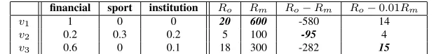
Table 1:Three possible latent vectors hypotheses for the definition ofbank#n#1

nius norm of difference between the two matrices is minimized:

v u u t

X

i

X

j

ˆ Xij−Xij

2

(2)

In effect, LSA allows missing and observed words to equally impact the objective function. Given the inherent short length of the sentences, LSA (equa-tion 2) allows for much more potential influence from missing words rather than observed words (99.9% cells are 0 in X). Hence the contribution of the observed words is significantly diminished. Moreover, the true semantics of the concept defini-tions is actually related to some missing words, but such true semantics will not be favored by the objec-tive function, since equation 2 allows for too strong an impact byXˆij = 0foranymissing word. There-fore the LSA model, in the context of short texts, is allowing missing words to have a significant “un-controlled” impact on the model.

2.1 An Example

The three latent semantics profiles in table 1 il-lustrate our analysis for topic models and LSA. As-sume there are three dimensions: financial, sports, institution. We useRv

o to denote the sum of related-ness between latent vectorvand all observed words; similarly,Rv_m is the sum of relatedness between the vectorvand all missing words. The first latent vec-tor (generated by topic models) is chosen by maxi-mizingRobs = 600. It suggestsbank#n#1is only related to thef inancialdimension. The second la-tent vector (found by LSA) has the maximum value of Robs −Rmiss = −95, but obviously the latent vector is not related tobank#n#1at all. This is be-cause LSA treats observed words and missing words equally the same, and due to the large number of missing words, the information of observed words is lost:Robs−Rmiss≈ −Rmiss. The third vector is the ideal semantics profile, since it is also related to theinstitutiondimension. It has a slightly smaller Robs in comparison to the first vector, yet it has a substantially smallerRmiss.

In order to favor the ideal vector over other vec-tors, we simply need to adjust the objective

func-tion by assigning a smaller weight toRmisssuch as: Robs−0.01×Rmiss. Accordingly, we use weighted matrix factorization (Srebro and Jaakkola, 2003) to model missing words.

3 The Proposed Approach

3.1 Weighted Matrix Factorization

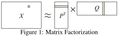
The weighted matrix factorization [WMF] ap-proach is very similar to SVD, except that it allows for direct control on each matrix cellXij. The model factorizes the original matrix X into two matrices such thatX ≈P>Q, whereP is aK×M matrix, andQis aK×N matrix (figure 1).

The model parameters (vectors in P andQ) are optimized by minimizing the objective function:

X

i

X

j

Wij(P·,i·Q·,j−Xij)2+λ||P||22+λ||Q||22 ₍₃₎

where λ is a free regularization factor, and the weight matrix W defines a weight for each cell in X.

Accordingly,P·,iis aK-dimension latent seman-tics vector profile for wordwi; similarly,Q·,j is the K-dimension vector profile that represents the sen-tencesj. Operations on these K-dimensional vec-tors have very intuitive semantic meanings:

(1) the inner product ofP·,i andQ·,j is used to ap-proximate semantic relatedness of wordwiand sen-tencesj: P·,i ·Q·,j ≈ Xij, as the shaded parts in Figure 1;

(2) equation 3 explicitly requires a sentence should not be related to its missing words by forcingP·,i· Q·,j = 0for missing wordsXij = 0.

(3) we can compute the similarity of two sentences sj andsj0 using the cosine similarity betweenQ_·,j,

Q·,j0.

The latent vectors in P andQare first randomly initialized, then can be computed iteratively by the following equations (derivation is omitted due to limited space, which can be found in (Srebro and Jaakkola, 2003)):

P·,i=

QW˜(i)Q>+λI−1QW˜(i)X>_i,·

Q·,j=

PW˜(j)P>+λI

−1

PW˜(i)X·,j

Figure 1: Matrix Factorization

where W˜(i) = diag(W·,i) is an M ×M diagonal

matrix containingith row of weight matrixW. Sim-ilarly, W˜(j) = diag(W·,j) is an N ×N diagonal matrix containingjth column ofW.

3.2 Modeling Missing Words

It is straightforward to implement the idea in Sec-tion 2.1 (choosing a latent vector that maximizes Robs −0.01×Rmiss) in the WMF framework, by assigning a small weight for all the missing words and minimizing equation 3:

Wi,j=

1, ifXij6= 0

wm, ifXij= 0 (5)

We refer to our model as Weighted Textual Matrix Factorization [WTMF].1

This solution is quite elegant: 1. it explicitly tells the model that in general all missing words should not be related to the sentence; 2. meanwhile latent semantics are mainly generalized based on observed words, and the model is not penalized too much (wm is very small) when it is very confident that the sentence is highly related to a small subset of missing words based on their latent semantics pro-files (bank#n#1definition sentence is related to its missing wordscheck loan).

We adopt the same approach (assigning a small weight for some cells in WMF) proposed for rec-ommender systems [RS] (Steck, 2010). In RS, an incomplete rating matrixRis proposed, where rows are users and columns are items. Typically, a user rates only some of the items, hence, the RS system needs to predict the missing ratings. Steck (2010) guesses a value for all the missing cells, and sets a small weight for those cells.

Compared to (Steck, 2010), we are facing a differ-ent problem and targeting a differdiffer-ent goal. We have a full matrixXwhere missing words have a 0 value, while the missing ratings in RS are unavailable – the values are unknown, henceRis not complete. In the RS setting, they are interested in predicting individ-ual ratings, while we are interested in the sentence

1_{An efficient way to compute equation 4 is proposed in}

(Steck, 2010).

semantics. More importantly, they do not have the sparsity issue (each user has rated over 100 items in the movie lens data2) and robust predictions can be made based on the observed ratings alone.

4 Evaluation for SS

We need to show the impact of our proposed model WTMF on the SS task. However we are faced with a problem, the lack of a suitable large evaluation set from which we can derive robust observations. The two data sets we know of for SS are: 1. human-rated sentence pair similarity data set (Li et al., 2006) [LI06]; 2. the Microsoft Research Paraphrase Cor-pus (Dolan et al., 2004) [MSR04]. The LI06 data set consists of 65 pairs of noun definitions selected from the Collin Cobuild Dictionary. A subset of 30 pairs is further selected by LI06 to render the sim-ilarity scores evenly distributed. While this is the ideal data set for SS, the small size makes it impos-sible for tuning SS algorithms or deriving significant performance conclusions.

On the other hand, the MSR04 data set comprises a much larger set of sentence pairs: 4,076 training and 1,725 test pairs. The ratings on the pairs are binary labels: similar/not similar. This is not a prob-lem per se, however the issue is that it is very strict in its assignment of a positive label, for example the following sentence pair as cited in (Islam and Inkpen, 2008) is rated not semantically similar:

Ballmer has been vocal in the past warning that Linux is a threat to Microsoft.

In the memo, Ballmer reiterated the open-source threat to Microsoft.

We believe that the ratings on a data set for SS should accommodate variable degrees of similarity with various ratings, however such a large scale set does not exist yet. Therefore for purposes of evaluat-ing our proposed approach we devise a new frame-work inspired by the LI06 data set in that it com-prises concept definitions but on a large scale.

4.1 Concept Definition Retrieval

We define a new framework for evaluating SS and project it as a Concept Definition Retrieval (CDR) task where the data points are dictionary definitions. The intuition is that two definitions in different

dic-2_{http://www.grouplens.org/node/73, with 1M data set being}

tionaries referring to the same concept should be as-signed large similarity. In this setting, we design the CDR task in a search engine style. The SS algorithm has access to all the definitions in WordNet (WN). Given an OntoNotes (ON) definition (Hovy et al., 2006), the SS algorithm should rank the equivalent WN definition as high as possible based on sentence similarity.

The manual mapping already exists for ON to WN. One ON definition can be mapped to sev-eral WN definitions. After preprocessing we obtain 13669 ON definitions mapped to 19655 WN defini-tions. The data set has the advantage of being very large and it doesn’t require further human scrutiny.

After the SS model learns the co-occurrence of words from WN definitions, in the testing phase, given an ON definitiond, the SS algorithm needs to identify the equivalent WN definitions by comput-ing the similarity values between all WN definitions and the ON definition d, then sorting the values in decreasing order. Clearly, it is very difficult to rank the one correct definition as highest out of all WN definitions (110,000 in total), hence we use ATOPd,

area under the TOPKd(k) recall curve for an ON definitiond, to measure the performance. Basically, it is the ranking of the correct WN definition among all WN definitions. The higher a model is able to rank the correct WN definition, the better its perfor-mance.

LetNdbe the number of aligned WN definitions for the ON definition d, andN_dk be the number of aligned WN definitions in the top-k list. Then with a normalized k ∈ [0,1], TOPKd(k) and ATOPd is defined as:

TOPKd(k) =Ndk/Nd

ATOPd= Z 1

0

TOPKd(k)dk

(6)

ATOPdcomputes the normalized rank (in the range of[0,1]) of aligned WN definitions among all WN definitions, with value 0.5 being the random case, and 1 being ranked as most similar.

5 Experiments and Results

We evaluate WTMF on three data sets: 1. CDR data set using ATOP metric; 2. Human-rated Sen-tence Similarity data set [LI06] using Pearson and Spearman Correlation; 3. MSR Paraphrase corpus [MSR04] using accuracy.

The performance of WTMF on CDR is com-pared with (a) an Information Retrieval model (IR) that is based on surface word matching, (b) an n-gram model (N-n-gram) that captures phrase overlaps by returning the number of overlapping ngrams as the similarity score of two sentences, (c) LSA that uses svds() function in Matlab, and (d) LDA that uses Gibbs Sampling for inference (Griffiths and Steyvers, 2004). WTMF is also compared with all existing reported SS results on LI06 and MSR04 data sets, as well as LDA that is trained on the same data as WTMF. The similarity of two sentences is computed by cosine similarity (except N-gram). More details on each task will be explained in the subsections.

To eliminate randomness in statistical models (WTMF and LDA), all the reported results are aver-aged over 10 runs. We run 20 iterations for WTMF. And we run 5000 iterations for LDA; each LDA model is averaged over the last 10 Gibbs Sampling iterations to get more robust predictions.

The latent vector of a sentence is computed by: (1) using equation 4 in WTMF, or (2) summing up the latent vectors of all the constituent words weighted by Xij in LSA and LDA, similar to the work reported in (Mihalcea et al., 2006). For LDA the latent vector of a word is computed byP(z|w). It is worth noting that we could directly use the es-timated topic distributionθjto represent a sentence, however, as discussed the topic distribution has only non-zero values on one or two topics, leading to a low ATOP value around 0.8.

5.1 Corpus

The corpus we use comprises three dictionaries WN, ON, Wiktionary [Wik],3 Brown corpus. For all dictionaries, we only keep the definitions without examples, and discard the mapping between sense ids and definitions. All definitions are simply treated as individual documents. We crawl Wik and remove the entries that are not tagged as noun, verb, adjec-tive, or adverb, resulting in220,000entries. For the Brown corpus, each sentence is treated as a docu-ment in order to create more coherent co-occurrence values. All data is tokenized, pos-tagged4, and

lem-3

http://en.wiktionary.org/wiki/Wiktionary:Main Page 4

Models Parameters Dev Test

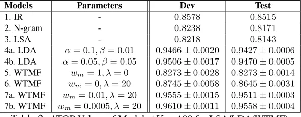
1. IR - 0.8578 0.8515 2. N-gram - 0.8238 0.8171 3. LSA - 0.8218 0.8143 4a. LDA α= 0.1, β= 0.01 0.9466±0.0020 0.9427±0.0006 4b. LDA α= 0.05, β= 0.05 0.9506±0.0017 0.9470±0.0005 5. WTMF wm= 1, λ= 0 0.8273±0.0028 0.8273±0.0014 6. WTMF wm= 0, λ= 20 0.8745±0.0058 0.8645±0.0031 7a. WTMF wm= 0.01, λ= 20 0.9555±0.0015 0.9511±0.0003 7b. WTMF wm= 0.0005, λ= 20 0.9610±0.0011 0.9558±0.0004 Table 2:ATOP Values of Models (K= 100for LSA/LDA/WTMF)

matized5. The importance of words in a sentence is estimated by the TF-IDF schema.

All the latent variable models (LSA, LDA, WTMF) are built on the same set of cor-pus: WN+Wik+Brown (393,666 sentences and 4,262,026words). Words that appear only once are removed. The test data is never used during training phrase.

5.2 Concept Definition Retrieval

Among the 13669 ON definitions, 1000 defini-tions are randomly selected as a development set (dev) for picking best parameters in the models, and the rest is used as a test set (test). The performance of each model is evaluated by the average ATOPd value over the 12669 definitions (test). We use the subscript set in ATOPset to denote the average of ATOPdof a set of ON definitions, whered∈ {set}. If all the words in an ON definition are not covered in the training data (WN+Wik+Br), then ATOPdfor this instance is set to 0.5.

To compute ATOPd for an ON definition effi-ciently, we use the rank of the aligned WN definition among a random sample (size=1000) of WN tions, to approximate its rank among all WN defini-tions. In practice, the difference between using 1000 samples and all data is tiny for ATOPtest(±0.0001), due to the large number of data points in CDR.

We mainly compare the performance of IR, N-gram, LSA, LDA, and WTMF models. Generally results are reported based on the last iteration. How-ever, we observe that for model 6 in table 2, the best performance occurs at the first few iterations. Hence for that model we use the ATOPdevto indicate when to stop.

5

http://wn-similarity.sourceforge.net, WordNet::QueryData

5.2.1 Results

Table 2 summarizes the ATOP values on the dev and test sets. All parameters are tuned based on the dev set. In LDA, we choose an optimal combination ofαandβfrom{0.01,0.05,0.1,0.5}.In WTMF, we choose the best parameters of weightwm for miss-ing words andλ for regularization. We fix the di-mensionK = 100. Later in section 5.2.2, we will see that a larger value ofKcan further improve the performance.

WTMF that models missing words using a small weight (model 7b withwm = 0.0005) outperforms the second best model LDA by a large margin. This is because LDA only uses10observed words to infer a100dimension vector for a sentence, while WTMF takes advantage of much more missing words to learn more robust latent semantics vectors.

The IR model that works in word space achieves better ATOP scores than N-gram, although the idea of N-gram is commonly used in detecting para-phrases as well as machine translation. Applying TF-IDF for N-gram is better, but still the ATOPtestis not higher:0.8467. The reason is words are enough to capture semantics for SS, while n-grams/phrases are used for a more fine-grained level of semantics.

We also present model 5 and 6 (both are WTMF), to show the impact of: 1. modeling missing words with equal weights as observed words (wm = 1) (LSA manner), and 2. not modeling missing words at all (wm = 0) (LDA manner) in the context of WTMF model. As expected, both model 5 and model 6 generate much worse results.

0.0001 0.0005 0.001 0.005 0.01 0.05 0.94

0.945 0.95 0.955

w_m

ATOP

WTMF

Figure 2:missing words weightwmin WTMF

50 100 150 0.94

0.945 0.95 0.955

K

ATOP

WTMF LDA

Figure 3:dimensionKin WTMF and LDA

that allowing for equal impact of both observed and missing words is not the correct characterization of the semantic space.

5.2.2 Analysis

In these latent variable models, there are several essential parameters: weight of missing wordswm, and dimensionK. Figure 2 and 3 analyze the impact of these parameters on ATOPtest.

Figure 2 shows the influence ofwm on ATOPtest values. The peak ATOPtestis aroundwm= 0.0005, while other values ofwm (exceptwm = 0.05) also yield high ATOP values (better than LDA).

We also measure the influence of the dimension K = {50,75,100,125,150} on LDA and WTMF in Figure 3, where parameters for WTMF arewm= 0.0005, λ = 20, and for LDA are α = 0.05, β = 0.05. We can see WTMF consistently outperforms LDA by an ATOP value of0.01in each dimension. Although a larger K yields a better result, we still use a100due to computational complexity.

5.3 LI06: Human-rated Sentence Similarity

We also assess WTMF and LDA model on LI06 data set. We still use K = 100. As we can see in Figure 2, choosing the appropriate parameterwm could boost the performance significantly. Since we do not have any tuning data for this task, we present Pearson’s correlationrfor different values ofwmin Table 3. In addition, to demonstrate that wm does not overfit the 30 data points, we also evaluate on

30 pairs 35 pairs

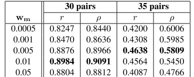
wm r ρ r ρ

0.0005 0.8247 0.8440 0.4200 0.6006 0.001 0.8470 0.8636 0.4308 0.5985 0.005 0.8876 0.8966 0.4638 0.5809

0.01 0.8984 0.9091 0.4564 0.5450

0.05 0.8804 0.8812 0.4087 0.4766

Table 3:Differentwmof WTMF on LI06 (K= 100)

the other 35 pairs in LI06. Same as in (Tsatsaronis et al., 2010), we also include Spearman’s rank order correlationρ, which is correlation of ranks of simi-larity values . Note thatrandρare much lower for 35 pairs set, since most of the sentence pairs have a very low similarity (the average similarity value is 0.065 in 35 pairs set and 0.367 in 30 pairs set) and SS models need to identify the tiny difference among them, thereby rendering this set much harder to predict.

Using wm = 0.01 gives the best results on 30 pairs while on 35 pairs the peak values of r and ρ happens when wm = 0.005. In general, the cor-relations in 30 pairs and in 35 pairs are consistent, which indicateswm = 0.01 orwm = 0.005does not overfit the 30 pairs set.

Compared to CDR, LI06 data set has a strong preference for a largerwm. This could be caused by different goals of the two tasks: CDR is evaluated by the rank of the most similar ones among all can-didates, while the LI06 data set treats similar pairs and dissimilar pairs as equally important. Using a smallerwmmeans the similarity score is computed mainly from semantics of the observed words. This benefits CDR, since it gives more accurate similarity scores for those similar pairs, but not so accurate for dissimilar pairs. In fact, from Figure 2 and Table 2 we see thatwm = 0.01 also produces a very high ATOPtestvalue in CDR.

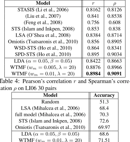
Table 4 shows the results of all current SS models with respect to the LI06 data set (30 pairs set). We cite their best performance for all reported results.

Model r ρ STASIS (Li et al., 2006) 0.8162 0.8126

(Liu et al., 2007) 0.841 0.8538 (Feng et al., 2008) 0.756 0.608 STS (Islam and Inkpen, 2008) 0.853 0.838 LSA (O’Shea et al., 2008) 0.8384 0.8714 Omiotis (Tsatsaronis et al., 2010) 0.856 0.8905 WSD-STS (Ho et al., 2010) 0.864 0.8341 SPD-STS (Ho et al., 2010) 0.895 0.9034 LDA (α= 0.05, β= 0.05) 0.8422 0.8663 WTMF (wm= 0.005, λ= 20) 0.8876 0.8966 WTMF (wm= 0.01, λ= 20) 0.8984 0.9091

Table 4: Pearson’s correlationrand Spearman’s corre-lationρon LI06 30 pairs

Model Accuracy

Random 51.3 LSA (Mihalcea et al., 2006) 68.4 full model (Mihalcea et al., 2006) 70.3 STS (Islam and Inkpen, 2008) 72.6 Omiotis (Tsatsaronis et al., 2010) 69.97

LDA (α= 0.05, β= 0.05) 68.6 WTMF (wm= 0.01, λ= 20) 71.51

Table 5:Performance on MSR04 test set

5.4 MSR04: MSR Paraphrase Corpus

Finally, we briefly discuss results of applying WTMF on MSR04 data. We use the same pa-rameter setting used for the LI06 evaluation set-ting since both sets are human-rated sentence pairs (λ = 20, wm = 0.01, K = 100). We use the train-ing set of MSR04 data to select a threshold of sen-tence similarity for the binary label. Table 5 sum-marizes the accuracy of other SS models noted in the literature and evaluated on MSR04 test set.

Compared to previous SS work and LDA, WTMF has the second best accuracy. It suggests that WTMF is quite competitive in the paraphrase recognition task.

It is worth noting that the best system on MSR04, STS (Islam and Inkpen, 2008), has much lower cor-relations on LI06 data set. The second best system among previous work on LI06 uses Spearman cor-relation, Omiotis (Tsatsaronis et al., 2010), and it yields a much worse accuracy on MSR04. The other works do not evaluate on both data sets.

6 Related Work

Almost all current SS methods work in the high-dimensional word space, and rely heavily on word/sense similarity measures, which is knowledge based (Li et al., 2006; Feng et al., 2008; Ho et al., 2010; Tsatsaronis et al., 2010), corpus-based (Islam

and Inkpen, 2008) or hybrid (Mihalcea et al., 2006). Almost all of them are evaluated on LI06 data set. It is interesting to see that most works find word sim-ilarity measures, especially knowledge based ones, to be the most effective component, while other fea-tures do not work well (such as word order or syn-tactic information). Mihalcea et al. (2006) use LSA as a baseline, and O’Shea et al. (2008) train LSA on regular length documents. Both results are con-siderably lower than word similarity based methods. Hence, our work is the first to successfully approach SS in the latent space.

Although there has been work modeling latent se-mantics for short texts (tweets) in LDA, the focus has been on exploiting additional features in Twit-ter, hence restricted to Twitter data. Ramage et al. (2010) use tweet metadata (author, hashtag) as some supervised information to model tweets. Jin et al. (2011) use long similar documents (the article that is referred by a url in tweets) to help understand the tweet. In contrast, our approach relies solely on the information in the texts by modeling local missing words, and does not need any additional data, which renders our approach much more widely applicable.

7 Conclusions

We explicitly model missing words to alleviate the sparsity problem in modeling short texts. We also propose a new evaluation framework for sentence similarity that allows large scale tuning and test-ing. Experiment results on three data sets show that our model WTMF significantly outperforms existing methods. For future work, we would like to compare the text modeling performance of WTMF with LSA and LDA on regular length documents.

Acknowledgments

We would like to thank the anonymous reviewers for their valuable comments and suggestions to improve the quality of the paper.

References

David M. Blei, Andrew Y. Ng, and Michael I. Jordan. 2003. Latent dirichlet allocation. Journal of Machine Learning Research, 3.

William Dolan, Chris Quirk, and Chris Brockett. 2004. Unsupervised construction of large paraphrase cor-pora: Exploiting massively parallel news sources. In

Proceedings of the 20th International Conference on Computational Linguistics.

Christiane Fellbaum. 1998. WordNet: An Electronic Lexical Database. MIT Press.

Jin Feng, Yi-Ming Zhou, and Trevor Martin. 2008. Sen-tence similarity based on relevance. InProceedings of IPMU.

Thomas L. Griffiths and Mark Steyvers. 2004. Find-ing scientific topics. Proceedings of the National Academy of Sciences, 101.

Chukfong Ho, Masrah Azrifah Azmi Murad, Rabiah Ab-dul Kadir, and Shyamala C. Doraisamy. 2010. Word sense disambiguation-based sentence similarity. In

Proceedings of the 23rd International Conference on Computational Linguistics.

Thomas Hofmann. 1999. Probabilistic latent semantic indexing. InProceedings of the 22nd annual interna-tional ACM SIGIR conference on Research and devel-opment in information retrieval.

Eduard Hovy, Mitchell Marcus, Martha Palmer, Lance Ramshaw, and Ralph Weischedel. 2006. Ontonotes: The 90% solution. InProceedings of the Human Lan-guage Technology Conference of the North American Chapter of the ACL.

Aminul Islam and Diana Inkpen. 2008. Semantic text similarity using corpus-based word similarity and string similarity. ACM Transactions on Knowledge Discovery from Data, 2.

Ou Jin, Nathan N. Liu, Kai Zhao, Yong Yu, and Qiang Yang. 2011. Transferring topical knowledge from auxiliary long texts for short text clustering. In Pro-ceedings of the 20th ACM international conference on Information and knowledge management.

David Kauchak and Regina Barzilay. 2006. Paraphras-ing for automatic evaluation. In Proceedings of the Human Language Technology Conference of the North American Chapter of the ACL.

Thomas K Landauer, Peter W. Foltz, and Darrell Laham. 1998. An introduction to latent semantic analysis.

Discourse Processes, 25.

Mirella Lapata and Regina Barzilay. 2005. Automatic evaluation of text coherence: Models and representa-tions. InProceedings of the 19th International Joint Conference on Artificial Intelligence.

Yuhua Li, Davi d McLean, Zuhair A. Bandar, James D. O Shea, and Keeley Crockett. 2006. Sentence similar-ity based on semantic nets and corpus statistics. IEEE Transaction on Knowledge and Data Engineering, 18. Xiao-Ying Liu, Yi-Ming Zhou, and Ruo-Shi Zheng. 2007. Sentence similarity based on dynamic time warping. InThe International Conference on Seman-tic Computing.

Rada Mihalcea, Courtney Corley, and Carlo Strapparava. 2006. Corpus-based and knowledge-based measures of text semantic similarity. InProceedings of the 21st National Conference on Articial Intelligence.

James O’Shea, Zuhair Bandar, Keeley Crockett, and David McLean. 2008. A comparative study of two short text semantic similarity measures. In Proceed-ings of the Agent and Multi-Agent Systems: Technolo-gies and Applications, Second KES International Sym-posium (KES-AMSTA).

Daniel Ramage, Susan Dumais, and Dan Liebling. 2010. Characterizing microblogs with topic models. In Pro-ceedings of the Fourth International AAAI Conference on Weblogs and Social Media.

Nathan Srebro and Tommi Jaakkola. 2003. Weighted low-rank approximations. InProceedings of the Twen-tieth International Conference on Machine Learning. Harald Steck. 2010. Training and testing of

recom-mender systems on data missing not at random. In

Proceedings of the 16th ACM SIGKDD International Conference on Knowledge Discovery and Data Min-ing.

George Tsatsaronis, Iraklis Varlamis, and Michalis Vazir-giannis. 2010. Text relatedness based on a word the-saurus.Journal of Articial Intelligence Research, 37. Liang Zhou, Chin-Yew Lin, Dragos Stefan Munteanu,