Munich Personal RePEc Archive
Breaking Bad in Bourbon Country: Does
Alcohol Prohibition Encourage
Methamphetamine Production?
Fernandez, Jose and Gohmann, Stephan and Pinkston,
Joshua
University of Louisville, Economics Department, University of
Louisville, Economics Department, University of Louisville,
Economics Department
25 August 2015
Breaking Bad in Bourbon Country: Does Alcohol Prohibition Encourage
Methamphetamine Production?
Jose Fernandez
University of Louisville
jose.fernandez@louisville.edu
Stephan Gohmann
University of Louisville
steve.gohmann@louisville.edu
Joshua C. Pinkston
University of Louisville
josh.pinkston@louisville.edu
November 2016
Acknowledegements: We would like to thank Zachary Breig, Scott Cunningham, John Graves, Matt Harris, Dan
Rees, Alex Tabarrok, as well as the conference/seminar participants at the American Society of Health Economists
in Philadelphia, the Society of Labor Economsts meetings in Seattle, Vanderbilt Empirical Applied Micreconomics
Festival, Southern Economic Association Conference in Tampa, American Economic Association Conference in
Philadelphia, the Association of Private Enterpise Education Conference, and Epi-hour at the University of
Abstract
This paper examines the influence of local alcohol prohibition on the prevalence of
methamphetamine labs. Using multiple sources of data for counties in Kentucky, we compare
various measures of meth manufacturing in wet, moist, and dry counties. Our preferred estimates
address the endogeneity of local alcohol policies by exploiting differences in counties’ religious
compositions between the 1930s, when most local-option votes took place, and recent years.
Even controlling for current religious affiliations, religious composition following the end of
national Prohibition strongly predicts current alcohol restrictions. We carefully examine the
validity of our identifying assumptions, and consider identification under alternative
assumptions. Our results suggest that the number of meth lab seizures in Kentucky would
1
Breaking Bad in Bourbon Country: Does Alcohol Prohibition Encourage
Methamphetamine Production?
This paper examines the influence of alcohol prohibition on the number of
methamphetamine (meth) labs in Kentucky. We carefully control for observable heterogeneity
between counties, and then address the remaining endogeneity of local alcohol laws. Our
preferred estimates exploit variation in religious affiliations in the 1930s, when most local-option
votes took place, that is not explained by current religious affiliations; however, we also consider
alternative identifying assumptions. In each case, our results suggest that local alcohol
prohibition increases in the prevalence of meth labs.
After the Federal prohibition of alcohol sales and production was repealed in 1933, some
states permitted localities to adopt local-option ordinances. Kentucky is one of 12 states that still
contain jurisdictions that prohibit sales of alcohol. Over a fourth of the 120 counties in Kentucky
are “dry”, meaning that all sales of alcohol are banned in the county. In contrast, “wet” counties
in Kentucky allow the sale of alcohol; “moist” counties contain wet jurisdictions, but are
otherwise dry; and “limited” counties only allow the sale of alcohol by the drink in certain types
of restaurants.
Miron and Zwiebel (1995) argue that alcohol bans flatten the punishment gradient for
alcohol drinkers to engage in other illicit activities, encouraging illicit drug use by raising the
relative price of a substitute. Consumers in dry jurisdictions can only purchase alcohol if they
drive to a jurisdiction that allows alcohol sales, or if they make an illegal local purchase.1 In
1
2
addition to introducing the risk of criminal penalties and asset forfeiture, alcohol transactions
with illegal dealers may provide consumers with more information about illicit drugs than they
would have otherwise.
Most previous empirical work is consistent with the idea that illegal drugs are substitutes
for alcohol. Conlin, Dickert‐Conlin, and Pepper (2005) find that a change in the status of Texas
counties from dry to wet lowers drug-related mortality by approximately 14 percent. DiNardo
and Lemieux (2001) find that higher minimum drinking ages reduce alcohol consumption by
high school seniors, but increase marijuana consumption. Crost and Guerrero (2012) find that
alcohol consumption increases and marijuana use falls at age 21, and Deza (2015) finds that hard
drug use also decreases at 21. Anderson, Crost, and Rees (2014) find that marijuana is a
substitute for alcohol, and that legalizing medical marijuana is associated with a decrease in
traffic fatalities.
On the other hand, Pacula (1998) finds that increases in beer taxes are associated with
less drinking and less marijuana use among young adults, consistent with the two goods being
complements. Yörük and Yörük (2011) find that marijuana use increases at age 21; however,
their results are strongest for a subsample that used alcohol, cigarettes or marijuana at least once
since the previous interview. Crost and Rees (2013) examine the same data and find no evidence
of complementarity between marijuana and alcohol.
Access to alcohol can also have indirect effects on other crimes. Carpenter (2005) finds
that zero-tolerance drunk driving policies reduce property crime among 18-21 year old males by
3.4 percent and reduce the incidence of nuisance crimes. Anderson et al. (2014) find an
association between establishments serving alcohol by the drink and violent crime. Other studies
3
find that higher alcohol excise taxes reduce alcohol consumption as well as certain types of
property and violent crime (See Carpenter & Dobkin, forthcoming for a full survey).
We contribute to the literature on the consequences of prohibition by considering the
effects of alcohol restrictions on meth lab seizures in Kentucky. On one level, our work can be
seen as contributing to the discussion of whether alcohol and illegal drugs are substitutes or
compliments. An advantage of our study is that we do not rely on self-reported drug use or
counts of drug arrests reported by law enforcement. As we argue in the next section, the counts
of meth labs we use should be less affected by potentially endogenous law enforcement behavior
than arrest data.2
On a more direct level, our work focuses on an outcome that has important implications
for public health, the production and use of methamphetamine. In a systematic review of the
literature on health consequence of meth use, Marshall and Werb (2010) find that users are more
likely to have suicidal ideation, eating disorders, paranoia, and mortality from overdose. The
production of methamphetamine not only places the “cooks” in danger from explosions, burns
and chemical injuries; but also creates an environmental hazard. Kentucky’s Department for
Environmental Protection reports that the average remediation cost is roughly $5,000 per lab,
with some clean-ups costing over $20,000.3
Gonzales, Mooney, and Rawson (2010) report that meth use in the United States
increased threefold between 1997 and 2007. Weisheit and Wells (2010) find that Kentucky has
one of the highest rates of meth lab seizures in the country, with 15.24 labs seized per 100,000
2
We also consider other outcomes, including various counts of drug arrests. We consider ER visits for burns as an alternative measure that is completely independent of law enforcement and illuminates a cost of local, amateur meth production. While our results using arrest data should be taken with a grain of salt, they are consistent with our results for meth labs, and they suggest that the negative effects of prohibition extend to other drugs.
3
4
residents between 2004 and 2008.4 They suggest that meth labs may be as prevalent as they are
in Midwestern and Southeastern states because distance from the Mexican border raises the costs
of imported meth relative to locally produced products.5 Cunningham et al. (2010) support this
conclusion, reporting that methamphetamine purity falls with distance from the borders with
Mexico and Canada, which is consistent with local demand being met by production in small
local labs. Kentucky’s location, therefore, suggests that its 120 counties are an excellent setting
to study the effects of alcohol restrictions on meth use and production.
Of course, local alcohol laws are likely endogenous. Toma (1988) argues that
local-options give voters an opportunity to increase the price of alcohol by increasing the cost of
obtaining it. Yandle (1983) points out that both bootleggers and Baptists have historically
supported alcohol bans: Baptists for religious reasons and bootleggers for economic reasons. In
both cases, local alcohol laws would be affected by the religious, cultural, and economic
characteristics of the area. Restrictions may also be enacted in response to local public health
concerns or other problems related to alcohol such as the incidence of drunk driving.
Our analysis begins with a careful treatment of observed heterogeneity between counties.
All of our estimates control for a wide array of geographic, demographic, economic and cultural
characteristics. Furthermore, we consider the robustness of our results to additional control
variables, functional form assumptions, and sample restrictions based on observable
characteristics. If anything, we find that adjusting for observable differences strengthens the
association between local-option status and the prevalence of meth labs.
4
Between 2004 – 2008 the ten states with the highest meth lab seizure rates (from highest to lowest) were Missouri, Arkansas, Iowa, Tennessee, Indiana, Kentucky, Alabama, Oklahoma, Kansas, and Mississippi. 5
5
We account for remaining unobserved heterogeneity using two different approaches, each
of which relies on different identifying assumptions. First, our preferred approach exploits
variation in religious composition shortly after the end of national prohibition that is independent
of counties’ current religious composition. We show that religious composition from the 1930s,
when most local option laws were passed, strongly predicts current wet/dry status; and we
perform multiple tests of the validity of our exclusion restrictions. Our second approach to
unobservable differences follows Oster (Forthcoming) and Altonji, Elder, and Taber (2005b)
(referred to as AET, 2005b), replacing exclusion restrictions with the assumption that selection
on observables is informative about selection on unobservables.
I.
Data
Our primary data are a panel of meth lab seizures and local-option ordinances for
Kentucky counties from 2004 to 2010. The lab seizure counts are from the DEA’s National
Clandestine Laboratory Register.6 The DEA provides the physical street addresses for all meth
labs seized as a public service due to the public health risk from chemical contamination. An
advantage of these data is that they do not depend solely on arrests or other law enforcement
interventions. The DEA also lists labs that are accidentally discovered following a fire or
explosion. Furthermore, the significant negative externalities associated with meth labs,
especially the unpleasant chemical odors, result in additional discoveries that are likely
independent of the intensity of local enforcement efforts.
In contrast, arrest data are known to suffer from potentially endogenous measurement
error (Levitt, 1998; Lott Jr & Whitley, 2003; Pepper, Petrie, & Sullivan, 2010). Reported arrest
6
6
rates are a function of the crime rates, the enforcement rates and the reporting behavior of local
law enforcement. When we compare arrest data from the FBI’s UCR and the Kentucky State
Police, we find some evidence that errors in the data vary with local option status. For example,
the correlation between the reported arrests for drug categories that are common to the two
databases varies with wet/dry status, even when we control for other county characteristics.7
Furthermore, the DEA data show at least one meth lab is discovered in over 18% of county/year
observations in which the UCR records no arrests for manufacturing or sales of any “other
nonnarcotic” drug, which includes methamphetamine.
County-level local-option ordinance data are provided by the Kentucky Department of
Alcoholic Beverage Control.8 In 2010, Kentucky had 32 wet counties, 39 dry counties, 20 moist
counties and 29 counties with limited alcohol access. For the sake of simplicity, we treat counties
with limited alcohol access as dry counties in our analysis, which should work against finding
effects of local alcohol bans.9
As a robustness check, we also collect drug-related arrest data from the FBI Uniform
Crime Reports (UCR) and the Kentucky State Police. Both sources include reported arrests
related to the sales, manufacturing and possession of “other nonnarcotic” drugs, which include
methamphetamine; and synthetic narcotics, which includes prescription opioids. The Kentucky
State Police data also provide reported arrests for meth-related crimes, including manufacturing,
7
Both datasets record arrests related to synthetic narcotics and “other nonnarcotic” drugs. Methamphetamine is in the “other” category. For both categories, the raw correlation between the reports in the UCR and the KSP databases is higher in wet counties than in dry, which is consistent with less accurate reporting in dry counties. Controlling for county characteristics explains much of this difference for “other” drugs; however, the differences in reporting accuracy for synthetic narcotics persist (and increase) when we control for county characteristics. 8
http://www.abc.ky.gov/ 9
7
sales, possession, dump sites, and unlawful possession of precursors. We use the sum of reported
meth-related incidents as a dependent variable in our robustness checks.
Similar to national trends, meth lab seizures in Kentucky fell by 50 percent between 2004
and 2007, but increased more than three-fold by 2010. As seen in Figure 1, the highest rates of
meth lab seizures occur in the southern counties bordering Tennessee and in the center of the
state. Comparing Figure 1 with Figure 2, which shows wet/dry status, there appears to be a
relationship between dry status and meth lab seizures. The mean lab seizure rate is 2.17 per
100,000 residents in wet, 2.26 in moist, and 3.92 in dry counties (see Table 1). The means for
moist counties are consistent with Campbell et al. (2009) who find that alcohol bans have smaller
effects when a jurisdiction is less geographically isolated.
We use county-level demographic variables from the U.S. Census and American
Community Survey. As suggested by Yandle (1983) and Strumpf and Oberholzer‐Gee (2002),
the demographic composition of voters influences local-option ordinances. Counties are more
likely to adopt restrictive alcohol policies as population, income, percent black, and percent
college educated decrease; or as poverty and unemployment increase.
Finally, we use data from Haines (2004) on religious membership in 1936 to capture
religious attitudes at the time of the initial wet/dry votes following the end of Federal
Prohibition. We control for current religious attitudes using data from the Association of
Religion Data Archives (2000, 2010). As a robustness check, we examine the sensitivity of our
results to the inclusion of controls for religious composition in 1990.
Table 1 shows the means of several key variables and how they vary by local-option
status. Wet counties are more densely populated on average than dry counties. Wet counties also
8
the observable differences between wet and dry counties, many of which are statisticaly
significant at a 5 percent level, the adoption of local-option ordinances should not be treated as
exogenous. Note also that religious participation and the share of Baptists, both of which are
associated with restrictive alcohol policies, have increased across all county types since 1936.10
II.
Estimation
To determine the robustness of our results we use four different estimation methods. The
first two methods address observable heterogeneity between counties. The next two address
unobservable differences that may be correlated with wet and dry status.11
Observable Heterogeneity
First, we consider an ordinary least squares model with year fixed effects and
county-level demographics to estimate the treatment effect:
𝑀𝑀𝑀ℎ𝐶𝐶𝐶𝐶𝑀𝐶𝑟𝑀𝑀𝑖𝑖 =𝛼𝑖+ 𝛾𝛾𝑀𝑟𝑀𝛾𝛾𝑖𝑖 +𝑋𝑖𝑖𝛽+𝑀𝑖𝑖
The year fixed effects, 𝛼𝑖, control for time-varying changes that affected the entire state. We
cannot include county fixed effects because we only observe a few changes in wet/dry status
during our sample period.12
The matrix 𝑋𝑖𝑖 consists of controls for geographic, demographic, economic and religious
characteristics. Following Strumpf and Oberholzer-Gee (2002), we include indicators for
bordering surrounding states and having a wet neighbor. We also control for latitude, longitude
10
Strumpf and Oberholzer-Gee (2002) study local prohibition ordinances between 1930 and 1940. They find Baptists, Presbyterians, and Methodists are more likely to support local prohibition; but Catholics, Episcopalians, and Lutherans are more likely to support legalized liquor.
11
All of these methods use linear models for the incidence of meth labs and other outcome variables. Estimates from Poisson count models, which can be found in the appendix, are qualitatively similar to the simpler linear specifications we present in the text.
12
9
and their interaction; access to interstate highways; and the ratio of residents working in the
county to total county employment.13 The demographic characteristics in 𝑋𝑖𝑖 are county
population; population density; and the percentages of the population who are married, male,
black, under age 21 and over 65. Economic controls include median household income; female
labor-force participation; the poverty rate; the percent of children receiving TANF; and the
percentages of acres dedicated to crops and pasture. Finally, we control for the percent of the
population belonging to a religious congregation, that percent squared, the number of Baptists,
and the interaction of the Baptist population with the percent black.14
The variables of interest in the regressions are the county alcohol 𝛾𝑀𝑟𝑀𝛾𝛾𝑖𝑖 variables. We
use three sets of measures for local-option status. The first are dummy variables indicating
whether the county is wet, moist or dry, with dry being the omitted category. The second
measure exploits variance between moist counties by measuring the percent of the county
population that lives in a wet jurisdiction. This variable equals one in wet counties and zero in
dry counties. Lastly, we use the number of liquor stores per 100,000 residents as an alternative
measure of wetness that is not based on the state local-option data.15
Our second estimation method is propensity score matching, which controls for observed
heterogeneity more flexibly than OLS. Propensity scores also allow us to identify and exclude
observations that are not comparable to any observation in another treatment group. For
example, the counties that contain Louisville and Lexington are wet, more densely populated and
13
A higher ratio of residents to total county employment suggests more isolation. This variable is constructed using data on commuting patterns from the American Community Survey.
14
Religion data from the 1930s suggest that black and white Baptists have different views on alcohol prohibition; however, the data from more recent years do not separate Baptists as clearly along racial lines.
15
10
otherwise different from any dry county in Kentucky. Additionally, a few dry counties are so
geographically isolated and sparsely populated that they are not comparable to any wet county.
The matching estimates we present only evaluate binary treatment variables. Specifically,
we perform this analysis for two groupings: wet vs dry and moist vs dry. We also estimated
multinomial treatment variables using inverse probability weighting instead of matching. The
estimates based on inverse probability weighting, which we report in the appendix, are similar to
those produced by the simpler matching estimates presented in the text.
Unobserved Heterogeneity
We use two approaches to address the likely unobserved heterogeneity among counties in
our sample. First, we exploit variation in religious membership following Prohibition that is not
correlated with current religious composition. A flurry of local-option votes occurred shortly
after the repeal of Prohibition in 1933. Since 1940, local option votes have become less common.
We find that per capita religious membership in 1936 and its square strongly predict current wet
status. All of our regressions include the current religion variables described above to ensure that
the instruments do not proxy for present day beliefs, which would compromise the credibility of
our exclusion restrictions.
For the IV estimation with discrete treatment groups, we only consider wet versus dry,
and group the moist counties into the dry category. Our instruments cannot identify wet and
moist as separate treatments.16 This grouping works against our finding an effect of alcohol bans
as some counties in the dry group contain moist counties, which are dry, but have wet
jurisdictions.
16
11
Additionally, we continue to restrict the sample for our IV estimates, excluding counties
with propensity scores that approach one or zero. We believe any attempt to identify exogenous
variation is more plausible if it doesn’t compare Louisville and the Cinncinnati suburbs to
racially homogeneous, isolated counties with a predicted probability of dry greater than 0.999.
For the sake of comparison, we also present analogous OLS results for the restricted sample.
Our identification strategy is unique in the literature on alcohol restrictions, which has
previously been dominated by difference-in-difference estimation based on changes in local
option laws (E.g., Baughman, Conlin, Dickert-Conlin, and Pepper (2001); Conlin et al. (2005)).
The advantage of our IV approach is that it does not require us to assume that local policy
changes are independent of time-varying unobservables. The disadvantage is that we must
assume that religious composition in the 1930s is not correlated with current unobserved county
characteristics, conditional on current religious composition and other observed characteristics.
Our approach finds some support in the work of Strumpf and Oberholzer-Gee (2002), who not
only use religion to capture local tastes for prohibition, but also argue that changes in local
alcohol laws are endogenous.
The Validity of Exclusion Restrictions
We address the possibility that counties’ religious compositions in the 1930s have
persistent correlations with unobserved county characteristics that are not captured by current
religion or other variables in a few ways. First, we consider the robustness of our results to the
addition of controls for religious composition in the 1990s and polynomials in the estimated
12
omitted variables.17 Motiviated by the possibility that counties with greater observable
differences likely have more unobservable differences, we also consider robustness to changes in
our sample restrictions based on extreme values of the propensity score.
We then examine the validity of our instruments using an approach discussed in Altonji,
Elder and Taber (2005a; 2005b). Considering instruments for Catholic high school attendance,
they regress various outcomes on proposed instruments using a sample of students who almost
never attend Catholic high school (public school eighth graders), eliminating the possibility that
these estimated coefficients are due to the instruments’ effects on Catholic high school
attendance. Non-zero coefficient estimates for instruments in that sample, therefore, reflect a
covariance between the instruments and unobservables, suggesting the instruments are not
valid.18
We execute the same test using a sample of counties that were dry as late as 1994, 10
years before our sample period began. These counties are still dry or moist in over 96 percent of
our observations. Two previously dry counties became wet between 1994 and 2004, and another
two became wet in 2009; however, these changes in treatment happened recently enough that
they should not have been caused by religious composition in 1936.19 Therefore, any apparent
effect our instruments have in this subsample cannot operate through the instruments’ effects on
wet status, even in the few cases where wet status is not zero.
17
We also considered potential bias due to enforcement efforts by adding the rate of property crime arrests as a regressor. The resulting changes in our coefficient estimates and the first-stage 𝐹 statistics were neglible, even though property crime is potentially endogenous in our context. These results are available upon request. 18
AET (2005b) reject the instruments used previously in the Catholic schooling literature, including the
contemporary share of Catholics in the local population. Our identification strategy resembles that of Cohen-Zada and Elder (2009) who use the historic shares of Catholics as an instrument for Catholic high school attendance, controlling for contemporary Catholic shares. When they perform the test of AET (2005b), they fail to reject the validity of historic Catholic shares as an instrument.
19
13
Proportional Selection on Obsevables and Unobservables
Finally, we use the proportional selection approach of Oster (2016), who extends AET
(2005b), to consider the amount of selection on unobservables that would be required to explain
away the entire effect suggested by our OLS estimates. This approach avoids the use of
exclusion restrictions; however, it does not provide point estimates. Instead, it simply tells us
whether some part of the effect implied by our OLS coefficients is likely to be causal.
AET (2005b) argue that the amount of selection on observable variables is informative
about the amount of selection on unobservables.20 If observable and unobservable characteristics
were drawn at random from the set of all relevant characteristics, then selection on observables
and unobservables should be equal; however, AET (2005b) argue that selection on
unobservables should be less than selection on observables when observable variables are chosen
to capture relevant variation. Therefore, we compare the amount of selection on unobservables
that would be needed to explain our OLS coefficients to the estimated selection on observables.
As the ratio of selection on unobservables to observables approaches or exceeds one, it becomes
increasingly likely that part of the covariance identified by our OLS coefficients reflects a causal
effect.
One difference between AET (2005b) and Oster (2016) is that Oster (2016) allows the
maximum possible 𝑅2 to be bounded below 1. This feature is important in our context because
counting the number of meth labs discovered in a calendar year necessarily introduces variance
from any underlying, “true” rate of meth lab discovery. To see this point, note that counting from
February to January would produce slightly different numbers than counting from January to
December. Even when we regress the meth lab rates on year and county fixed effects, county
20
14
time trends, and all of our time-varying control variables, we can’t produce an 𝑅2 over 0.764.
Therefore, we set the maximum 𝑅2 at 0.8 when performing the proportional selection test.21
III. Results
As described above, we examine the number of meth lab siezures per capita using three
different measures of county wet/dry status and four estimation techniques. The three wet/dry
measures are dummy variables for wet and moist counties, the percent of the population living in
a wet jurisdiction, and the number of liquor stores per capita. The four estimation techniques are
ordinary least squares, propensity score matching, instrumental variables, and the proportional
selection approach of Oster (2016).
Table 2presents the OLS and propensity score results for our primary outcome variable,
DEA Meth Lab Seizures. Column 1 shows the OLS results using observations from all counties,
while estimates in columns 2 through 4 exclude observations where the Pr (𝑤𝑀𝑀) approaches 0 or
1.22 Column 4 presents OLS results that compare wet counties to dry and and moist counties,
facilitating comparison to our IV results.
All models find that legal access to alcohol is associated with fewer meth labs per
capita.23 The OLS estimates using the full sample suggest that wet counties have 1.47 (0.61)
fewer meth labs and moist counties have 1.03 (0.53) fewer meth labs than dry counties. In the
middle panel, the coefficient estimate for the percent wet treatment variable is 1.17 (0.60). In the
bottom panel, the point estimates for liquor stores per capita are also negative, but are not
statistically significant.
21
We use psacalc.ado, which Oster wrote to accompany her paper, to perform this test in Stata. 22
Specifically, we exclude observations where the Pr(𝑤𝑀𝑀) is above 0.99999 or below 0.00001. 23
15
Next, we use propensity score matching to estimate the treatment effects. The basic
common support restriction applied in this table reduces the sample size from 840 to 800
observations.24 As mentioned above, we estimate propensity score treatment effects for wet vs
dry and moist vs dry separately, with samples of 656 and 369 observations.25
The propensity score matching results in the second column of Table 2 again suggest that
allowing alcohol sales in a county reduces the prevalence of meth labs. Wet counties have 2.48
(0.34) fewer labs and moist counties have 2.10 (0.41) fewer labs than dry counties. Both point
estimates are statistically significant at the 1 percent level. As seen in Appendix Table 3, these
results are not sensitive to estimating separate binomial treatments. If anything, the estimated
treatment effects increase in magnitude as we control for observable heterogeneity more
carefully.
For the sake of comparison, the third and fourth columns in Table 2 present OLS results
using the restricted sample that excludes counties that are off the common support. This results
in slightly larger coefficient estimates compared to OLS using the full sample; however, the
estimated coefficients in the first panel are still much smaller than the propensity score estimates.
When wet counties are compared to both dry and moist counties, as they are by our instrumental
variables estimates, the coefficient on the wet county indicator falls to -1.08 (0.57).
Table 3 presents estimates that use religious composition from the 1930s as instrumental
variabels. The first column presents results using the same sample and control variables as the
last three columns of Table 2. The other columns in Table 3 investigate the robustness of our
results by adding control variables or varying the estimation sample. The smallest first-stage 𝐹
24
These results are robust to applying a stricter common support restriction that limits attention to observations with a Pr (𝑛𝑛𝑀𝑤𝑀𝑀) between 0.03 and 0.9999.
25
Estimation results that use inverse probability weighting to estimate multinomial treatment effects are
16
statistic in the table is 51.5, consistent with religions composition in the 1930s being a strong
predictor of current local option status, despite our controls for current religious composition.26
The results in Table 3 uniformly suggest that local alcohol access decreases the
prevalence of meth labs in a county. Focusing on the main specification in the first column, wet
counties are estimated to have 2.38 (1.14) fewer meth labs per 100,000 than moist or dry
counties. The estimated effect of the percent wet treatment variable is -2.58 (1.28). Finally, the
IV estimates suggest that liquor stores have a statistically significant, negative effect on the
number of meth labs, with a coefficient of -0.092 (0.045). While the IV coefficients are all much
larger than their OLS analogs in Table 2, the IV coefficient on the wet county treatment variable
is only slightly larger than the propensity score estimate.27
Taken at face value, these estimates suggest that repealing all alcohol prohibition in
Kentucky would decrease the total number of meth lab seizures in the Commonwealth by almost
43 labs per year. This translates to a 34.5 percent decrease in the prevalence of meth labs
statewide, and a 59.8% percent decrease in moist and dry counties.
The Validity of our Instrumental Variables
The remaining columns of Table 3 consider the robustness of our IV estimates as an
informal means of assessing the validity of our instruments. If religious composition in the 1930s
is correlated with some aspect of current culture that is not captured by our controls for current
religious composition, then adding controls for religion from the more recent past should affect
our results; however, the second column shows that the estimated effects of alcohol access
26
Using only the rate of religious membership in 1936 and its square as instruments means that tests of
overidentifying restrictions are not useful in our case. In previous drafts, we also used the number of Baptists and black Baptists as instruments, which arguably made overidentification tests more meaningful; however, the historic Baptist variables were relatively weak instruments. In any case, none of our overidentification tests
suggest a problem for our main results. 27
17
change very little when measures of religious composition in 1990 are added to the regressions.28
As an additional test for correlation with omitted variables, the third column adds a cubic
polynomial in the estimated propensity score. The results suggest that, if anything, controlling
for observed differences in a more flexible manner increases the estimated effects of local
alcohol access.
The final colums of Table 3 restrict the sample further, excluding wet counties with a
predicted Pr(𝑛𝑛𝑀𝑤𝑀𝑀) < 0.03 and dry counties with a predicted Pr(𝑛𝑛𝑀𝑤𝑀𝑀) > 0.9999.29 If
our instruments are correlated with unobserved county characteristics, and unobservable
differences are more pronounced in counties that differ more along observable dimensions,
trimming counties based on extreme values of the propensity score should affect our estimates.
But the coefficients in the fourth and fifth columns are again similar to those in the first.30
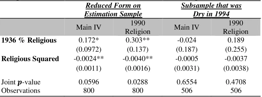
Table 4 presents a more formal evaluation of our instrumental variables. Following AET
(2005b), we first present the reduced form coefficients for our instruments using the main
estimate sample. We then present analogous coefficients estimated on a sample of counties that
were dry in 1994. As discussed in Section II, the estimates from the counties that were dry in
1994 can only reflect covariance between our instruments and unobserved county characteristics.
As expected, the reduced form coefficients in the first two columns are statistically
significant, suggesting that the number of meth labs increases with religious membership in 1936
at low levels of membership, but eventually decreases as membership rises.31 Adding controls
28
The variables added to the regressions in the second column are the percent of the population in 1990 that belonged to a religious congregation, that percent squared, and the number of Baptists in 1990.
29
The minimum Pr(𝑛𝑛𝑀𝑤𝑀𝑀) among dry counties is 0.034. The maximum among wet counties is 0.9998. 30
The fifth column adds both the religion variables from the second column and the propensity score polynomial from the third.
31
18
for religion in 1990, in addition to current religious composition, results in larger coefficients in
the second column, but the increase is not statistically significant.
More importantly, the coefficients on the 1936 religion variables are uniformly smaller in
the subsample that was dry in 1994, and they are neither individually nor jointly statistically
significant. The reduced-form coefficients in the main specification (first column) are several
times larger than the analogous estimates in the third column. Furthermore, we see a similar
pattern when we consider effects of our instruments on alternative outcomes such as ER visits
for burns or drug arrests (not shown). We find no evidence of covariance between our
instruments and unobservable county characteristics, regardless of which outcomes we consider.
Proportion of Selection on Unobservables
Our final estimation method considers the potential influence of unobserved county
characteristics without relying on exclusion restrictions. As discussed in Section II, we use the
approach of Oster (2016) to estimate the proportion of influence the unobservables would need
to have relative to observed characteristics to suggest that our OLS coefficients do not reflect any
causal effect. As the proportion approaches or exceeds one, it becomes increasingly reasonable
to believe we have identified some causal relationship, even if that relationship is smaller than
our point estimates.
Table 5 presents the OLS coefficients and proportion required for zero causal effect for
several regressions. The coefficients of proportionality are estimated assuming a maximum 𝑅2 of
0.8, which is nearly four times larger than any estimated 𝑅2 in the table.32 The regressions in the
first column were also presented in the last two columns of Table 2. The later columns add
control variables and vary the sample restrictions.
32
19
The results in Table 5 again suggest a causal effect of local alcohol access on the
prevalence of meth labs. Despite the coefficients in the first column being the most conservative
estimates in the table, we find that selection on unobservables would need to be roughly the same
as selection on observables before the entire OLS coefficient could be explained by unobservable
factors.
The case for a causal effect only grows stronger as we attempt to reduce omitted variable
bias or further restrict the sample based on observable differences. Adding controls for religious
composition in 1990 raises the OLS coefficients and coefficients of proportionality, but the
change is not dramatic. When we add a polynomial in the propensity score, we find that
unobservable differences would need to have 2.7 times the influence of the observable variables
in order to explain the coefficient on the wet dummy variable; and 1.5 times the influence of
observables to explain the coefficient on the percent living in a wet jurisdiction. If we further
restrict the sample to counties that are more observably similar, the coefficients of
proportionality for the wet county treatment variable continue to exceed two; and the coefficients
of proportionality for the percent treated suggest that selection on unobservables would need to
be several times larger than selection on observables to explain our OLS coefficients.
It’s worth noting that the negative coefficient in the lower panel of the fifth column
suggests that our controls for observable characteristics increase the estimated treatment effect.
This reflects the fact that our control variables do not uniformly mitigate the differences in meth
production between wet and dry counties. For example, our controls for geographic coordinates
and population reduce the coefficients on our treatment variables; however, adjusting for religion
(current or 1990) or many of our economic controls increases the estimated treatment effects. If
20
than our basic controls for geography and demographics, our OLS coefficients understate the
true causal effects, as suggested previously by our IV and propensity score estimates.
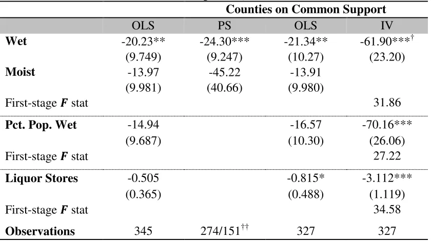
Alternative Outcome Measures
As a robustness check, we repeat our estimates using data on ER visits for burns, as well
as arrest data from the UCR and the Kentucky State Police (KSP). Burns can be viewed as an
alternative measure of meth production that is entirely independent of law enforcement
reporting.33 On the other hand, we view the arrest data with some suspicion; however, they do
provide alternative measures of local drug crime.
The production of meth involves corrosive, combustible chemicals and a heating element.
“Cooks” risk chemical and conventional burns. We obtained data on emergency room visits for
burns from chemicals or hot substances from the Kentucky Injury Prevention and Research
Center.34 As shown in Table 6, there is a consistent pattern of fewer burns per capita in wet
counties. The OLS estimates in both samples indicate roughly 20 fewer ER burn visits per
100,000 residents, which is similar to the propensity score estimate of 24.3 (9.2) fewer visits.
The magnitude of the reduction in burns increases dramatically when we use instrumental
variables. The coefficient for the wet treatment in the first panel is -61.9 (23.2), and the
coefficient on the percent wet is -70.2 (26.1). The IV coefficient on liquor stores per capita, -3.1
(1.1), also suggests that alcohol access reduces ER burn visits.
33
We have also examined data on hospital admissions for drug overdoses; however, the overdose data we’ve acquired so far contain a large number of censored values in order to protect patient confidentiality in small cells. Burns, being more common, are censored less often.
34
21
Table 7 presents results for three categories of drug arrests. The outcome in the first panel
is the rate of all meth-related incidents, as reported by the KSP.35 The outcome variables in the
second and third panels are the arrest rates for synthetic narcotics, including Oxycodone and
other prescription opiates, as reported by the UCR and the KSP.36
The results for total meth-related crimes in the first panel are very much consistent with
our main results. Least squares estimates using either the full or restricted samples find a
reduction in meth-related arrests of 20 to 22 per 100,000 residents in wet counties. The
propensity score estimates find larger reductions, with wet counties having 32.03 (9.29) fewer
meth-related arrests and moist counties having 27.63 (13.55) fewer arrests. The IV estimates find
that wet counties have 47.65 (19.25) fewer meth-related arrests. The IV estimates for the percent
wet and the liquor store treatment variables also find statistically significant reductions in
meth-related arrests when alcohol sales are allowed.
Given the systematic measurement error noted above, it is not surprising to see the results
for synthetic narcotic arrests vary somewhat between the UCR and the KSP data. That said, the
IV results in the second and third panels still paint a consistent picture, suggesting that alcohol
prohibition encourages the illegal use and distribution of prescription opiates, as well as crystal
meth. The coefficients on the wet treatment dummy suggest reductions of 28 to 35 arrests per
100,000. The coefficients on the percent wet vary from -31.1 (11.6) to -35.8 (18.6).
Our final outcome measure addresses the possibility that unobserved health trends are
associated with both the demand for illicit drugs and local alcohol policy. If poor population
health is a motivation for local prohibition, then we should observe “effects” on other health
measures. In Table 8, we report the effects of local-option status on childhood obesity as a
35
The meth-related crimes include dumpsites, possession, sales, paraphanellia, and meth labs. 36
22
falsification test. All of the estimates are close to zero, they vary in sign, and none of them are
statistically significant. Furthermore, we find similar results when using infant mortality as the
dependent variable (not shown), despite the potential effects of alcohol consumption on fetal
health.
Comments and Alternative Explanations
Although most of our results focus on supply-side measures, the observed effects could
still reflect the local demand for methamphetamine. The geographic position of Kentucky far
from the country’s borders and its sparse population lower the (private) costs of local production,
including production for personal use, relative to importation. According to the DEA,
methamphetamine and marijuana are the only illegal drugs that are easily produced by the users:
“A cocaine or heroin addict cannot make his own cocaine or heroin, but a methamphetamine
addict only has to turn on his computer to find a recipe identifying the chemicals and process
required for production of the drug.” (Keafe, 2001). Furthermore, Cunningham et al. (2010) find
that methamphetamine purity falls with distance from Mexico and Canada, which is consistent
with demand being met by small, amateur labs.
An alternative supply-side story is that meth labs may be more prevalent in dry counties
due to a longer history of illicit alcohol production. Experience producing “moonshine” may
result in greater knowledge about hiding labs, more skilled production, greater ability to
influence law enforcement, and more extensive networks for distributing illegal products. But
it’s not clear that these channels would result in a higher number of labs being discovered, even
if they did result in a higher volume of illicit production.37 If anything, greater experience with
37
23
illicit production would suggest that the number of meth labs would be undercounted to a greater
degree in dry counties, which would bias our estimates toward zero.
That said, we acknowledge that our estimated effects may be realized gradually following
a change in policy. Legal liquor sales would make alcohol more readily available, reducing the
benefits of illegal production and distribution of alcohol or other drugs. The relative costs of
producing, distributing and using methamphetamine would rise immediately; however, amateur
production by addicted users may change more slowly.
IV. Conclusion
We find strong evidence that local alcohol prohibition in Kentucky increases the
prevalence of methamphetamine labs in dry jurisdictions. Our results suggest that, if all counties
in Kentucky became wet, the number of meth labs statewide would be reduced by 34.5 percent.
Although we consider data on arrests to be less reliable than the DEA’s lab seizure data, our
results using drug arrests not only support those based on meth labs, but also suggest that the
negative consequences of alcohol prohibition extend to prescription optiates. Furthermore, we
find that local alcohol prohibition increases the prevalence of ER visits for burns, which is
consistent with local labs being run by poorly trained amateur “cooks.”
We address the likely endogeneity of local-option status using a novel set of instrumental
variables. There was a spate of votes in Kentucky following the end of national Prohibition with
relatively few votes since the 1940s. We find that the religious composition of counties in 1936
strongly predicts current wet/dry status, even controling for current religious composition. We
find support for our exclusion restrictions using the test of AET (2005b), as well less formal
tests. Furthermore, we use the approach of Oster (2016) to provide evidence of causal effects that
24
Our work adds to the literature documenting unintended consequences of restricting
access to alcohol. Our results are consistent with the work of Conlin et al. (2005), Dinardo and
Lemieux (2001), and others who have found evidence of substitution between alcohol and other
drugs. Our results support the idea that prohibiting the sale of alcohol lowers the relative cost of
participating in the market for illegal drugs.
Finally, our work has implications for policy aimed at reducing the harm caused by the
use and production of methamphetamine. The most notable policies intended to reduce meth
production have been restrictions on precursors. Even though studies of earlier interventions
(Cunningham & Liu, 2003, 2005; Dobkin & Nicosia, 2009) found that these policies had only
temporary effects on the supply of meth, most states and the Federal government had placed
restrictions on the purchase of pseudoephedrine (a common cold medicine) by 2006. The most
careful study we have seen of precursor restrictions, Dobkin, Nicosia, and Weinberg (2014),
estimates that the restrictions reduced the number of meth labs in a state by around 36 percent,
which is comparable to our estimate of the effect of ending local alcohol prohibition. Although
it’s not clear how well our results would generalize to other states or to substances other than
alcohol, our study provides an example in which liberalizing the treatment of one substance may
25
26
27
Table 1: Means of outcome and control variables
County Demographic Variables Wet Moist Dry
Meth lab seizures rate (DEA)a,b 2.17 2.26 3.92
Non-narcotic Drug Possession rate (UCR) 98.8 95.9 90.8
Non-narcotic Drug Sale/Manufacture rate (UCR) 76.8 89.0 91.9
All Meth Related Incidences (KSP) rate a,b 42.2 55.5 81.2
Property Crime Rate a,b,c 451 358 267
Violent Crime Rate a,b,c 101 79.9 60.8
ER Burns ratea 132 137 149
Population (1000’s) a,b,c 70.1 38.4 20.2
Population Density a,b,c 245 111 60.7
Median Household Income ($1000) a,b,c 40.4 37.2 32.5
Pct. Access to Interstate Highway a,b 40.1 43.0 21.6
Pct. Resident Workers/ Total Employment a,b,c 48.7 56.1 53.1
Pct. Black a,b,c 6.38 3.79 2.57
Pct. Children Obese 17.2 17.4 17.2
Pct. College a,b 16.3 15.6 11.5
Pct. Female Labor Force Participation a,b 34.1 32.4 30.0
Pct. Male a,b 49.0 49.0 49.6
Pct. Married a,b,c 54.0 55.5 56.5
Pct. Widowed a,b 7.13 7.28 8.16
Pct. Poverty a,b,c 17.7 19.3 21.4
Pct. Poverty under 18 years old a,b 24.3 25.2 27.9
Pct. Public Assistancea 2.64 2.72 2.93
Pct. Under 21 years old a,b 28.8 28.4 27.4
Pct. Over 65 years old a,b 12.6 12.9 14.4
Pct. Any Religion 53.1 50.8 50.5
Pct. Baptista,c 30.0 32.8 35.2
Pct. Baptist of All Religiona,c 56.6 65.7 67.4
Pct. Any Religion in 1936 a,b,c 38.2 30.6 26.9
Pct. Baptist in 1936 12.8 12.0 13.5
Pct. Black Baptist in 1936 a,b,c 3.30 2.61 1.56
Pct. Baptist of All Religion in 1936 a,b,c 34.8 38.5 49.3
Population in 1936 (1000’s) 37.1 27.7 15.9
Note: DEA = Drug Enforcement Agency, KSP = Kentucky State Police, and UCR = FBI Uniform Crime Report. County level demographics are collected from the American Community Survey. Religion characteristics in 1936 are collected from Hayes (2010) and contemporary religion data are collected from the Association of Statisticians of American Religious Bodies. All rates are calculated per 100,000 people in the county population. Equal means
t-test at α=.05 are conducted for each pair of groups. Significant outcomes are indicated: a = wet vs dry, b = moist vs
28
Table 2: Effect of Alcohol Access on DEA Meth Lab Seizures per 100,000. Controlling for Observable Heterogeneity.
Full Sample Counties on Common Support
OLS PS OLS OLS††
Wet -1.469** -2.482*** -1.505** -1.082*
(0.608) (0.336) (0.641) (0.566)
Moist -1.029* -2.100*** -1.093**
… (0.535) (0.413) (0.537)
𝑹𝟐 0.20 0.21 0.21
Pct. Pop. Wet -1.166*
… -1.167* …
(0.599) (0.635)
𝑹𝟐 0.20 0.21
Liquor Stores per cap -0.013
… -0.038 …
(0.025) (0.033)
𝑹𝟐 0.19 0.21
Observations 840 656/369† 800 800
Robust standard errors in parentheses. Propensity score estimates use Abadie–Imbens robust standard errors. *** p<0.01, ** p<0.05, * p<0.1
All specifications use current county demographic information, current religious organization membership, county latitude and longitude, interstate highway access, Census commuting patterns, state and dry county border dummies, and year fixed effects.
Common Support limits the sample to observations with Pr(𝑑𝐶𝑑) between 0.00001 and 0.99999.
†
Propensity score estimates are constructed by comparing wet vs dry (n=656) and moist vs dry (n=369) separately.
††
29
Table 3: Effects of Alcohol Access on DEA Meth Lab Seizures per 100,000. Using Religious Composition in 1936 as Instrumental Variables.
Added Controls Strict Common Support†
Main IV 1990 Religion
Prop. Score
Polynomial Main IV
Added Controls
Wet†† -2.377** -2.528** -3.118** -2.077* -2.477** (1.136) (1.152) (1.270) (1.077) (1.190) First-stage 𝑭stat 91.77 79.45 61.29 92.22 58.31
Pct. Pop. Wet -2.580** -2.274* -3.476** -2.348* -2.716**
(1.282) (1.347) (1.446) (1.208) (1.363)
First-stage 𝑭 stat 83.29 71.75 53.03 78.08 51.52
Liquor Stores -0.0917** -0.0940 -0.112** -0.0857* -0.118*
(0.0454) (0.0578) (0.0497) (0.0443) (0.0626) First-stage 𝑭
stat 119.78 75.35 109.39 118.89 60.77
Observations 800 800 800 749 749
Robust standard errors in parentheses. *** p<0.01, ** p<0.05, * p<0.1
All specifications control for the same county characteristics as in Table 2, including current religious composition. The instrumental variables are the percent of the population in 1936 who belong to a religious congregation, and that percent squared. The 1990 religion variables added in the second and fifth columns are the percent belonging to a congregation, that percent squared, and the number of Baptist adherents in the county. The third and fifth columns add a cubic polynomial in the estimated Pr (𝑛𝑛𝑀𝑤𝑀𝑀).
†
The stricter common support restriction in the last two columns drops observations from wet counties with a predicted Pr(𝑑𝐶𝑑) < 0.03, and from dry counties with Pr(𝑑𝐶𝑑) > 0.9999. The sample in the first three columns only limits attention to observations with Pr(𝑑𝐶𝑑) between 0.00001 and 0.99999.
††
30
Table 4: Effect of Instruments on Meth Labs in Counties that were Dry in 1994, Compared to Reduced Form Coefficients for Estimation Sample.
Reduced Form on Estimation Sample
Subsample that was Dry in 1994
Main IV 1990
Religion Main IV
1990 Religion
1936 % Religious 0.172* 0.303** -0.024 0.189
(0.0972) (0.137) (0.187) (0.255)
Religious Squared -0.0024** -0.0040** -0.0005 -0.0037
(0.0011) (0.0016) (0.0031) (0.0038)
Joint 𝒑-value 0.0596 0.0288 0.6554 0.4708
Observations 800 800 506 506
Robust standard errors in parentheses. *** p<0.01, ** p<0.05, * p<0.1
31
Table 5: Proportion of Selection on Unobservables Needed for Zero Treatment Effect
Primary Estimation Sample Strict Common Support
Main 1990 Religion
Prop. Score
Polynomial Main
1990 Religion
Prop. Score Polynomial
Wet -1.082* -1.102* -1.258** -1.268** -1.270** -1.210** (0.566) (0.573) (0.590) (0.559) (0.571) (0.583)
Estimated 𝑅2 0.209 0.209 0.211 0.220 0.221 0.224
Coefficient of Proportionality for Zero Effect
𝑅𝑚𝑚𝑚2 = 0.8 1.106 1.195 2.703 3.085 3.163 2.178
Pct. Pop. Wet -1.167* -1.213* -1.294* -1.557** -1.611** -1.518**
(0.635) (0.649) (0.670) (0.632) (0.661) (0.650)
Estimated 𝑅2 0.208 0.209 0.210 0.221 0.222 0.225
Coefficient of Proportionality for Zero Effect
𝑅𝑚𝑚𝑚2 = 0.8 0.946 1.102 1.492 22.399 -17.219 8.325
Observations 800 800 800 749 749 749
Robust standard errors in parentheses. *** p<0.01, ** p<0.05, * p<0.1
Regressions in the first column are the same as OLS regressions presented in third and fourth columns of Table 2. All specifications control for the same county characteristics as in previous tables, including current religious composition. The 1990 religion variables added in the second and fifth columns are the percent belonging to a congregation, that percent squared, and the number of Baptist adherents in the county. The third and sixth columns add a cubic polynomial in the estimated Pr(not wet).
32
Table 6: Effect of ER visits for Burns per 100,000
Counties on Common Support
OLS PS OLS IV
Wet -20.23** -24.30*** -21.34** -61.90***† (9.749) (9.247) (10.27) (23.20)
Moist -13.97 -45.22 -13.91
(9.981) (40.66) (9.980)
First-stage 𝑭 stat 31.86
Pct. Pop. Wet -14.94 -16.57 -70.16***
(9.687) (10.30) (26.06)
First-stage 𝑭 stat 27.22
Liquor Stores -0.505 -0.815* -3.112***
(0.365) (0.488) (1.119)
First-stage 𝑭 stat 34.58
Observations 345 274/151†† 327 327
Robust standard errors in parentheses. Propensity score uses Abadie–Imbens robust standard errors. *** p<0.01, ** p<0.05, * p<0.1
All specifications include current county demographic information, religious membership, county latitude and longitude, interstate highway access, Census commuting patterns, as well as state border and dry county border dummies. The IV specifications use religious membership for 1936 as instruments. Full Sample results use all Kentucky counties between 2004 – 2010. Common Support restricts the sample to include counties with overlapping propensity scores of the Pr(dry).
†
Moist counties are included with dry counties in this estimation.
††
33
Table 7: Effects of Alcohol Access on Drug Arrests,
Counties on Common Support
OLS PS OLS IV
Total Meth-related Arrests (KSP)
Wet -22.41** -32.03*** -20.58** -47.65** (8.762) (9.292) (8.644) (19.25)
Moist -14.99 -27.63** -14.42
(9.196) (13.55) (9.443)
Pct. Pop. Wet -17.62** -15.54* -49.00**
(8.695) (8.593) (21.74)
Liquor Stores -0.0510 -0.621 -1.741**
(0.366) (0.472) (0.758)
Total Synthetic Drug Arrests (UCR)
Wet -5.623 -3.127 -5.552 -28.41*** (4.182) (2.846) (4.294) (10.34)
Moist 8.227 -23.70* 8.986
(6.197) (12.90) (6.187)
Pct. Pop. Wet -5.599 -5.615 -31.06***
(4.155) (4.333) (11.59)
Liquor Stores 0.00698 -0.146 -1.104***
(0.159) (0.189) (0.413)
Total Synthetic Drug Arrests (KSP)
Wet -3.952 -17.45*** -1.455 -34.80** (9.577) (6.092) (9.571) (16.42)
Moist -7.249 -26.41*** -6.883
(7.066) (7.070) (6.979)
Pct. Pop. Wet -1.456 1.352 -35.77*
(9.544) (9.626) (18.60)
Liquor Stores 0.485 0.175 -1.271*
(0.446) (0.636) (0.661)
Robust standard errors in parentheses. Propensity score uses Abadie–Imbens robust standard errors. *** p<0.01, ** p<0.05, * p<0.1
All specifications include current county demographic information, religious membership, county latitude and longitude, interstate highway access, Census commuting patterns, as well as state border and dry county border dummies. The IV specifications use religious membership for 1936 as instruments. Full Sample results use all Kentucky counties between 2004 – 2010. Common Support restricts the sample to include counties with overlapping propensity scores of the Pr(dry).
†
Propensity score estimates are constructed by comparing wet vs dry (n=655) and moist vs dry (n=445) separately.
††
Moist counties are included with dry counties in this estimation
34
Table 8: Falsification Test: “Effects” on the Percent of Children who are Obese
Full Sample Counties on Common Support
OLS PS OLS IV
Wet 0.004 -0.004 0.006 -0.009†
(0.005) (0.004) (0.005) (0.009)
Moist -0.0004 0.0019 -0.002
(0.004) (0.0055) (0.004)
Pct. Pop. Wet 0.004 0.007 -0.0005
(0.005) (0.005) (0.0095)
Liquor Stores per cap 0.0001 -0.0002 -0.00003
(0.0002) (0.0002) (0.0003)
Observations 811 640/363†† 776 776
Robust standard errors in parentheses, except for propensity score which uses Abadie–Imbens robust standard errors. *** p<0.01, ** p<0.05, * p<0.1
All specifications use current county demographic information, current religious organization membership, county latitude and longitude, interstate highway access, Census commuting patterns, as well as state border and dry county border dummies. The instrumental variable specifications use religious organization membership for 1936 as instruments. Full Sample results use the full sample of Kentucky counties between 2004 – 2010. Common Support restricts the sample to include counties with overlapping propensity scores of the Pr(dry).
†
Moist counties are included with dry counties in this estimation.
††
35
Appendix 1: Means of outcome and control variables for Counties on the Common Support
County Demographic Variables Wet Moist Dry
Meth lab seizures Rate (DEA) a,b 2.34 2.26 3.79
Synthetic Narcotic Arrest Rate (KSP) 42.2 42.7 53.7
Synthetic Narcotic Possession Rate (UCR)a,b 29.9 36.5 23.4
Synthetic Narcotic Sale/Manufacture Rate (UCR) 18.5 25.2 21.1
Non-narcotic Drug Possession Rate (UCR) 98.0 95.9 90.8
Non-narcotic Drug Sale/Manufacture Rate (UCR) 77.2 89.0 91.3
All Meth Related Arrest Rate (KSP)a 44.9 55.5 76.3
Property Crime Arrest Rate a,b 390.1 385.3 272.0
Violent Crime Arrest Rate a,b 86.4 79.9 61.9
ER Burns Ratea 134.6 138.6 149.3
Population (1000’s) a,b 34.1 38.6 21.6
Population Density a,b 122.3 109.7 61.0
Median Household Income ($1000) a,b, c 37.9 35.9 30.9
Pct. Access to Interstate Highway a,b 32.2 43.0 20.2
Pct. Resident Workers/ Total Employment a,b, c 49.4 56.1 53.4
Pct. Black a,b, c 5.10 3.84 2.57
Pct. College a,b 14.1 15.3 11.2
Pct. Children Obese 16.9 17.2 17.3
Pct. Female Labor Force Participation a,b 37.6 36.1 34.1
Pct. Male a,b 49.1 49.0 49.4
Pct. Marrieda 55.5 56.1 57.3
Pct. Widowed a,b 7.29 7.31 8.06
Pct. Poverty a,b 17.7 19.0 21.7
Pct. Poverty under 18 years old a,b 23.7 24.2 28.0
Pct. Public Assistancea 3.02 3.04 3.59
Pct. Under 21 years olda,b 29.1 28.6 27.9
Pct. Over 65 years olda,b 12.6 12.8 14.0
Pct. Any Religion 51.9 50.8 49.3
Pct. Baptista,c 30.3 34.6 34.7
Pct. Baptist of All Religiona 58.9 65.7 66.7
Pct. Baptist in 1936 13.2 12.0 13.2
Pct. Black Baptist in 1936a,b 3.3 2.6 1.6
Pct. Any Religion in 1936a,b,c 37.4 30.4 26.5
Pct. Baptist of All Religion in 1936a,b 44.5 46.2 54.5
Population in 1936 (1000’s)a,b,c 22.1 27.4 16.6
Note: DEA = Drug Enforcement Agency, KSP = Kentucky State Police, and UCR = FBI Uniform Crime Report. Common Support restricts the sample to include counties with
36
Appendix 2: Poisson Count Models for Various Outcomes
Analogous to OLS Estimates on Common Support from Tables 2, 6 and 7 Meth Labs
(DEA)
ER Burn Visits
Meth Arrests (KSP)
Synth. Narcotic Arrests (UCR) (KSP)
Wet County -0.591*** -0.160*** -0.490*** -0.105 -0.0489
(0.202) (0.0324) (0.0651) (0.0693) (0.160)
Moist County -0.430*** -0.113 -0.426*** 0.156 -0.0857
(0.0796) (0.0752) (0.117) (0.112) (0.161)
Pct. Pop. Wet -0.528** -0.124*** -0.441*** -0.117** -0.0204
(0.211) (0.0347) (0.0718) (0.0522) (0.160)
Liquor Stores -0.0168 -0.00612*** -0.0173** 0.00430 0.00430
(0.0125) (0.000597) (0.00868) (0.0131) (0.0131)
Observations 800 327 800 800 800
Robust standard errors in parentheses. *** p<0.01, ** p<0.05, * p<0.1
37
Appendix 3: Inverse Propensity Score Weighting Estimates for Various Outcomes
Analogous to Propensity Score Matching Estimates from Tables 2, 6 and 7
Meth Labs (DEA)
ER Burn Visits
Meth Arrests (KSP) †
Synth. Narcotic Arrests† (KSP) (UCR)
Wet County -3.288*** -25.14 -39.13** -29.59*** -1.701
(0.544) (15.50) (16.22) (6.187) (4.960)
Moist County -2.012*** -23.58** -15.83 -16.79** 14.86*
(0.727) (10.50) (13.29) (7.268) (8.672)
Observations 770 317 770 770 770
Robust standard errors in parentheses. *** p<0.01, ** p<0.05, * p<0.1
All models control county demographic information, current religious organization membership, county latitude and longitude, interstate highway access, Census commuting patterns, as well as state border and dry county border dummies.The sample size is restricted to include counties with overlapping propensity scores.
†