Predictive Models for Disaggregate Stock Market Volatility

(1)

Munich Personal RePEc Archive

Predictive Models for Disaggregate Stock

Market Volatility

Chong, Terence Tai Leung and Lin, Shiyu

The Chinese University of Hong Kong, Nanjing University

8 November 2015

Online at

https://mpra.ub.uni-muenchen.de/68460/

(2)

Predictive Models for Disaggregate Stock Market Volatility

Terence Tai-Leung CHONG1

Department of Economics, The Chinese University of Hong Kong

and

Department of International Economics and Trade, Nanjing University

and

Shiyu LIN,

Department of Economics, The Chinese University of Hong Kong

8/11/2015

Abstract: This paper incorporates the macroeconomic determinants into the

forecasting model of industry-level stock return volatility in order to detect whether

different macroeconomic factors can forecast the volatility of various industries. To

explain different fluctuation characteristics among industries, we identified a set of

macroeconomic determinants to examine their effects. The Clark and West (2007)

test is employed to verify whether the new forecasting models, which vary among

industries based on the in-sample results, can have better predictions than the two

benchmark models. Our results show that default return and default yield have

significant impacts on stock return volatility.

Keywords: Industry level stock return volatility; Out-of-sample forecast; Granger

Causality.

JEL classifications: C12, G12

1

(3)

1. Introduction

The determinants of stock return volatility have long been studied over the past

two decades (Campbell, Lettau, Malkiel and Xu, 2001; Sohn, 2009). Although these

studies commonly look into a wide range of macroeconomic variables, their different

methodologies yield results that are hardly comparable. While some studies suggest

that macroeconomic factors have impacts on stock return volatility, others find such

evidence lacking. Schwert (1989) examines the relationships between stock return

volatility and economic activities using monthly data from 1857 to 1987. He finds

that inflation volatility predicts stock volatility for the period 1953–1987, money

growth volatility is a good predictor of stock return volatility, and industrial

production volatility weakly explains stock return volatility. Kearney and Daly (1998)

show that conditional inflation volatilities and interest rates have direct impacts on

Australian stock market volatility. Engle and Rangel (2008) also argue that volatility

in macroeconomic factors, such as inflation, short-term interest rates and GDP

growth, could explain the increase in stock market volatility.

In the literature, very few studies have examined the impact of macroeconomic

variables on stock return volatility at the industry level (Faff and Brailsford, 1999;

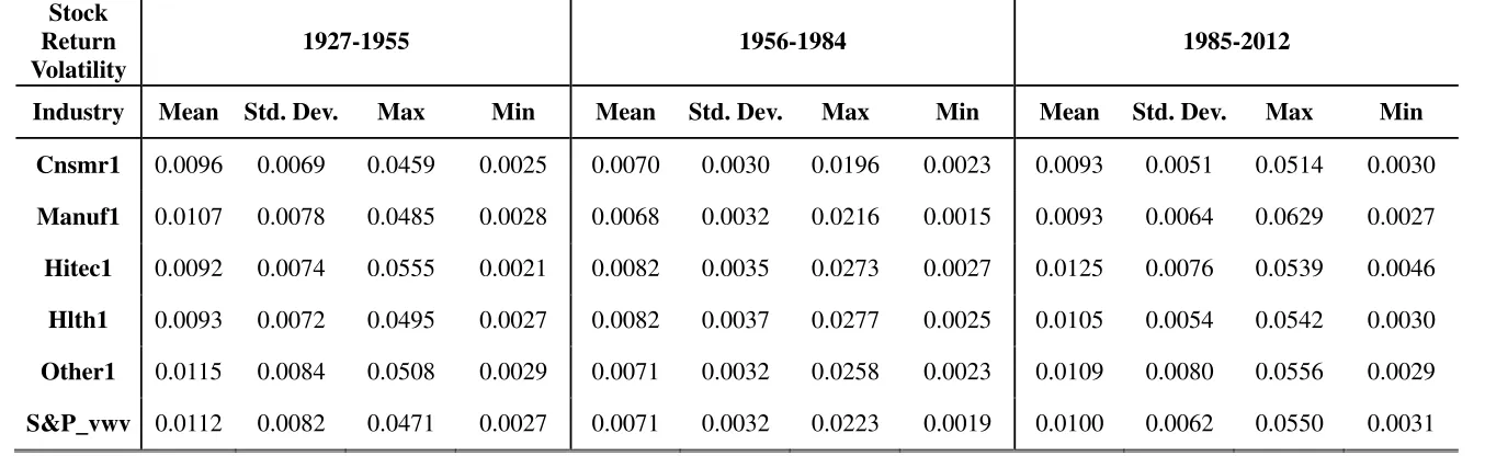
Hess, 2003). Figure 1 depicts the fluctuations of stock market volatility of the S&P

500 value-weighted market portfolio and major industries from 1927 to 2012. The

countercyclical characteristic of stock return volatility is largely consistent among

these major industries. However, since 2000, the stock return volatility of the Hitec1

(Business Equipment and Telecommunication) sector has increased, particularly

during the dot-com bubble, the 9/11 terrorist attacks, and the 2008 financial crisis. In

addition, the stock return volatility of Cnstr3 (Construction) is quite different from

(4)

different industries have different levels of sensitivity towards macroeconomic

factors.

Industry analysis contains important information for asset allocation, which

helps control portfolio risk by diversifying investments across various industries. The

objective of this paper is to investigate whether different macroeconomic factors can

forecast the volatility of various industries. A multi-factor augmented model is

constructed by adopting the main approaches in Schwert (1989) with U.S. stock

market data across different industries over the period 1927 to 2012. Paye (2012)

concludes that the macroeconomic variables Granger cause stock return volatility at

monthly horizons, and that the default return and default yield spread are the two

variables contributing the most. Following Paye (2012), we include explanatory

variables that reflect monetary policies (default return and default yield), economic

conditions (industrial production growth and its volatility) and price levels (inflation

rate).

The findings illustrate that for major industries, the aforementioned variables

have significant impacts on stock return volatility. Meanwhile, differences in the

impact of macroeconomic variables are evident among disaggregated industries.

These new forecasting models are empirically superior, based on the results of the

in-sample analysis. As for the out-of-sample analysis, the new forecasting models

perform better than the benchmark models constructed by auto-regressions or basic

settings for the aggregate market. However, the superiority is not exactly the same

(5)

The remainder of this paper is organized as follows. Section 2 reviews the

relevant literature on the differences in the fluctuations and macroeconomic

determinants of stock return volatility at the industry level. Section 3 describes the

variables and data. Sections 4 and 5 present the methodology and empirical results of

in-sample and out-of-sample analyses respectively. Section 6 concludes the paper.

2. Literature Review

The attempt to examine the different effects of macroeconomic factors on

volatility in different industries is mainly driven by the diverse characteristics of

industry-level volatility. Some industries are cyclical, such as the oil and gas industry

(Sadorsky, 2001) and durable equipment-based industries (machinery and

transportation equipment). Conversely, non-cyclical industries, such as food and

beverage, tobacco, and utilities (Campbell et al., 2001), sail through economic

downturns. Boudoukh et al. (1994) conclude that stock returns in non-cyclical

industries tend to co-vary positively with the expected inflation, while the reverse

holds for cyclical industries. According to Hess (2003), firms in sensitive sectors

underwent severe structural changes during the 1990s recession because of fierce

international competition and technological progress. Insensitive sectors, however,

did not face such significant challenges at the time.

Fama and French (1997) find substantial differences in factor sensitivities across

U.S. industries. As shown by Faff and Brailsford (1999), oil price movements have

varying effects on different industries. Specifically, while a significantly positive

sensitivity is spotted in diversified resources and the oil and gas industries, a

significantly negative sensitivity is observed in the transportation, paper and

(6)

Based on the investigation on the Pacific Stock Exchange (PSE) Technology 100

Index, the conditional volatilities of oil prices, the term premium, and the consumer

price index all have significant impacts on the conditional volatilities of technology

stock prices (Sadorsky, 2003).

A relatively large number of studies focus on the varying impacts of interest

rates and other factors in various industries. For example, Sweeney and Warga (1986)

perform regressions on the stock returns of 21 industry portfolios against the market

and a series of simple changes of long-term interest rates. They found that from 1960

to 1979, only stocks of electric utilities and those of the banking, finance and real

estate industries are consistently sensitive to interest rates. Dinenis and Staikouras

(1998) conclude that the effect of unanticipated changes in interest rates on

nonfinancial institutions is also statistically significant, but is substantially less

significant than the corresponding effect on financial institutions. Specifically, with

three-factor index model regressions, Oertmann et al. (2000) estimate interest rate

sensitivity by looking into various types of financial companies and industrial

corporations. Generally, the industrial corporations’ equity returns are positively

affected by interest rate changes. Oertmann et al. (2000) conclude that the

relationship commonly presumed negative between interest rate shifts and stock

returns is largely facilitated by financial companies in the market. Czaja and Scholz

(2007) use the term-structure model to examine the linkage between variables and

summarise the negative effects of the slope of term structure or term spread on stock

returns. The effects, nonetheless, vary among industries. For instance, the automobile

and utilities industries, which depend on large initial capital investments and

(7)

For variables reflecting price levels, the service sector tends to react more

sensitively to inflation surprises than the capital-intensive industrial sector does

(Hess, 2003). Specifically, the reaction of hotels to inflation shocks is more than two

time as strong as any other sector, as hotels may involve highly leveraged firms.

Retail-related sectors likewise are quite sensitive to inflation shocks, which may be

attributable to consumer behaviour. Comparatively, banks are only moderately

sensitive to inflation surprises.

3. Variables and Data

3.1 Explanatory Variables

Since countercyclical volatility may arise from investor uncertainty towards

economic status and risk premiums, observable variables correlating to these

channels are examined in the following analysis. This paper utilises the following

macroeconomic factors, which are sampled monthly from January 1927 to December

2012.

Industrial production growth (ipg)

This variable is defined as

1 ln( t )

t

ip ipg

ip_

 , where , the U.S. Industrial

Production Index, is sourced from the Board of Governors of the Federal Reserve

System. It measures movements in the level of output and highlights the structural

development of the economy.

Volatility of industrial production growth (ipgvol)

(8)

volatility of growth in U.S. industrial production . We estimate an

autoregressive model with 12-monthly dummy variables to evaluate the

monthly volatility of industrial production growth (



ˆ

_t2, from the following

regression). The volatility of industrial production is expressed as

12 12

1 1

t j jt i t i t j i

X  D  X_ 

 









 , (2)

where X_t denotes the monthly industrial production growth.

Default return spread (dfr)

This variable is the difference between returns from long-term corporate bonds

and long-term government bonds. Data (including the following two variables, dfy

and tms) are sourced from Goyal and Welch (2008), which was updated by Goyal

through 2012.

Default yield spread (dfy)

This variable is the difference between the yield on BAA-rated corporate bonds

and long-term U.S. government bonds.

Term spread (tms)

This variable is the difference between the long-term yield on government bonds

and the Treasury bill rate.

Factors representing price levels

(9)

This variable is defined as

1

ln( t )

t

ppi infl

ppi

 , where ppi_t is the producer price

index of month

t

. The ppi_tseries is sourced from the U.S. Bureau of Labor

Statistics website.

Industrial production growth and overall production growth provide useful

information about the uncertainty towards macroeconomic prospects. The growth of

the industrial production index can be consistent with the average growth of firms’

sales and cash flows (Chen, Roll and Ross, 1986). Humpe and Macmillan (2009)

find a positive correlation between the industrial production index and stock prices in

both American and Japanese markets. In addition, stock market volatility may

increase as industrial production volatility increases.

Paye (2012) argues that the most significant variables, in terms of Granger

causality, from macroeconomic factors to stock return volatility are default return,

default yield, and term spread. According to Chen et al. (1986), the default return has

a zero mean in a risk-neutral world. It can be considered a direct measure of the level

of risk aversion and implicit risk in the market’s stock pricing, as well as a reflection

of unanticipated movements in these risk levels. The default return reflects relative

preference in the bond market based on corporate and government bonds returns. A

higher default return indicates that corporate bond prices increase more compared to

government bond prices. This represents a relatively greater demand for corporate

bonds, which are riskier than government bonds. A higher default return corresponds

to a lower level of risk aversion and hence, a lower risk premium. Under the

assumption of countercyclical and asymmetric risk premium, prices and

(10)

anticipate stock return volatility to be negatively correlated with the default return.

The default yield spread responds aggressively at the onset of economic crises,

when default probabilities of corporate debt increase dramatically. The default yield

refers to the yield difference between BAA-rated corporate bonds and long-term U.S.

government bonds, and can be treated as another proxy for risk premium that is

calculated based on a company’s quality. When the yield difference between

BAA-rated corporate bonds and long-term U.S. government bonds is larger (i.e., the

BAA-rated companies may have relatively larger default risk), economy-wide stress

and subsequently a higher risk premium may result. Through the time-varying risk

aversion channel, stock return volatility also becomes correspondingly higher. Chen

et al. (1986) show evidence of a positive relationship between this default yield

spread and stock returns.

Term spread, which is the difference between the long-term yield on government

bonds and the Treasury bill rate, carries information about the changes in risk

premium and monetary policy during crises (Fornari and Mele, 2013). Chen et al.

(1986) suggest that this variable measures the unanticipated returns on long-term

government bonds. The growth of term spread indicates that the long-term

government bond yield increases more than the Treasury bill rate, and the demand

for long-term government bonds increases. Through the risk premium channel, both

the level of risk aversion and the amount of risk premium decrease. Therefore, the

term spread should have a negative impact on stock return volatility.

Table 1 presents the descriptive statistics of macroeconomic variables over the

period of 1927 to 2012. The Phillips and Perron unit root test is conducted for all

(11)

and Perron unit root test and calculated the associated Mackinnon approximate

p-value respectively. Since the null hypothesis of a unit root test for all variables is

rejected, we do not report the test results to conserve space.

3.2 Stock Return Volatility

This paper defines stock return volatility based on a classical definition of return

volatility (i.e., realised volatility obtained through sums of observed squared returns

within a reference period). This definition has been widely adopted (see, e.g.,

Anderson, Bollerslev and Diebold, 2007) since the pioneering work of Merton

(1980).

In this paper, the aggregate stock returns for comparison are the S&P 500

monthly returns (including all distributions) from a value-weighted market portfolio

(i.e., CRSP_VWRETD sourced from the Centre for Research in Security Prices

(CRSP)). The industry-level return comprises value-weighted returns from industry

portfolios obtained from the Kenneth R. French Data Library. From there, daily

returns of 5, 10, and 49 value-weighted industry portfolios are obtained based on

different degrees of industry classification. 9 of the 49 industries are omitted due to

missing observations. Those portfolios are therefore considered separately in this

study.

The realised volatility in each industry from January 1927 to December 2012 is

obtained from the standard deviation formula below:

2

, , ,

1

( )

(t)

1 t

N

j i t j t i

t

R R SRV

N



 





(12)

where SRV(t) is the stock return volatility in period

t

; R_{j i t}_{, ,} is the daily stock

return in industry j on the date i in period

t

; R_{j t}_, is the average return in

industry j in period

t

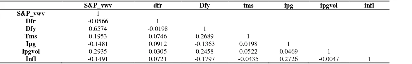
, and N_t is the number of trading days in this period.

The three panels in Table 2 report the industry information, including the mean

and the standard deviation of stock return volatility in different industries, as well as

the short names, definitions, and four-digit SIC codes that are used to assign firms to

5, 10, and 40 industries from French’s website. Numbers (1, 2, 3) following the short

names represent the degrees of classification, from general to disaggregated.

In other words, from the 5- to the 10- and the 40-industry classification, the

industries are becoming more disaggregated. For instance, Cnsmr1 in the 5-industry

classification contains Nodur2, Durbl2, and Shops2 in the 10-industry classification,

while Hitec1 in the 5-industry classification contains Hitec2 and Telcm2 in the

10-industry classification. Similarly, Nodur2 in the 10-industry classification consists

of some industries in the 40-industry classification, including Agric3, Toy3, Food3,

Books3, Clths3, Bldmt3, and Hshld3.

Table 2 reinforces the fact that industries have diverse volatility characteristics.

Some industries have higher levels of average stock return volatility. These industries

include Hitec1 (Business Equipment and Telecommunication), Durbl2 (Consumer

Durables), Toys3 (Recreation), Cnstr3 (Construction), Coal3 (Coal), and Rlest3

(Real Estate). The null hypothesis of Phillips and Perron unit root test is rejected in

all industries, indicating that persistence is not severe and our results provide credible

guidance.

(13)

volatility of the aggregate market (S&P_vwv) and that of the industries based on the

5-industry classification in three sub-periods are shown in Table 3. The first period

(1927–1955) covers the Great Depression, while the third period (1985–2012)

features the Great Moderation and the 2008 global financial crisis. The level of

volatility of the aggregate markets (Manuf1 and Other1) is higher than that of other

industries during the first period. Meanwhile, Hitec1 grows higher in volatility in the

third period. This evidence attests to the diverse fluctuations in stock return volatility

of those industries similar to Figure 1, which shows that the Hitec1 sector becomes

more volatile during the 21st century.

The correlation coefficients between stock return volatility at the aggregate level

and macroeconomic variables are shown in Table 4. The default yield, term spread,

and industrial production growth volatility correlate positively with the S&P 500

stock return volatility, while the default return, industrial production growth, and

inflation rate have weak and negative impacts on volatility. Moreover, we do not find

significant correlations among macroeconomic variables, reinforcing the credibility

of the results.

4. In-Sample Analysis

4.1 Model

The multi-factor forecasting model used in this paper is given by

6

, , , 1 ,

1

j t j j i j t i t j t i

SRV





SRV 



X







 



  , (4)

(14)

stands for the first-order lag of macroeconomic variables (i.e., default return, default

yield, term spread, industrial production growth, volatility of industrial production

growth, and inflation rate). The null hypothesis states that there is no Granger

causality, meaning that given a vector X_t₁_,the coefficients of macroeconomic

variables





0

can be tested using the F-test. Meanwhile, the t-test is used to

assess the significance of each macroeconomic determinant.

When





0

, the model becomes an AR (6) regression for each industry, which

is the benchmark model given by

6

, , , ,

1

j t j j i j t i j t i

SRV





SRV  u



 



 , (5)

where_{j i}_, is the coefficient associated with each lag of stock return volatility.

4.2 Results

Tables 5, 6, and 7 show the in-sample predictive regression results on a monthly

horizon of the 5-, 10- and 40-industry classifications respectively. For each industry,

the tables display the estimated slope coefficients



and their significance. Since all

macroeconomic variables are standardised prior to analysis, the coefficients reported

are measured in units of standard deviation.

In addition, the bottom parts of Tables 5 to 7 show the R-squared of the

predictive models and of the benchmark models, as well as the relative increase in

R-squared expressed as percentages and Granger causality test results for the

(15)

Table 5 depicts the in-sample predictive regression results for the S&P 500 and

5-industry classification, including Cnsmr1 (Consumer Goods), Manuf1

(Manufacturing, etc.), Hitec1 (Business Equipment, etc.), Hlth1 (Health Care, etc.),

and Other1. The results show that both default return and default yield have

significant effects on the volatility of the S&P 500 value-weighted stock returns. This

can also be found in all the five industries. The impact of default yield is relatively

larger on the stock return volatility in the consumer goods (Cnsmr1) and

manufacturing (Manuf1) industries, while the influences of default return on stock

return volatility are almost the same within the S&P 500 and the industries (except

Other1). For instance, a coefficient estimate of 0.083 implies that a one-standard

deviation shock to the default yield spread increases the volatility forecast of

manufacturing (Manuf1) industries in the subsequent period by 0.083 units. There is

no obvious evidence to show that other factors (i.e., term spread, industrial

production growth, volatility of industrial production growth, and inflation rate) have

significant impacts.

The null hypothesis of no Granger causality is rejected in all industries at the 5%

significance level. The R-squared of the model and benchmark model, and the

relative change are also reported. Cnsmr1 (Consumer Goods), Hlth1 (Health Care,

etc.), and Manuf1 (Manufacturing, etc.) show relatively greater increases in

R-squared after adding all macroeconomic factors to the benchmark AR (6) model.

To a large extent, the results of the coefficient estimates for these five main industries

are consistent with Paye (2012), who finds that the macroeconomic variables

Granger-cause stock return volatility at monthly horizons, and that the default return

(16)

With regards to a more disaggregated industry classification, Table 6 displays

the results of in-sample predictive regressions in 10 industries, which contain

Nodur2 (Non-Durable Goods), Durbl2 (Durable Goods), Enrgy2 (Oil, Gas, etc.)

and Shops2 (Wholesale, Retail, etc.). Similar to the results in 5 major industries, the

macroeconomic variables here Granger-cause stock return volatility in 10 industries.

However, industry differences become more apparent.

The effects of default return and default yield are significant among the

aforementioned 10 industries except Manuf2 (Manufacturing Industry), which is

not sensitive to the default return but reacts significantly to the default yield. Since

the production and business involved in the manufacturing industry generally

requires large initial investments and possess relatively longer profit cycles, this

industry may not be sensitive to the realised risk changes reflected by the return

difference between long-term corporate bonds and long-term government bonds.

However, it is highly sensitive to the changes of long-term expected risk reflected in

the yield difference between BAA-rated corporate bonds and long-term U.S.

government bonds.

In addition, the stock return volatility of the Hitec2 (Business Equipment)

industry reacts significantly to the term spread changes, probably owing to the

relatively higher risk and R&D cost of business equipment firms. The volatility of

Utils2 (Utilities) co-varies with the volatility of industrial production growth. This is

evident given that utilities contain electric, gas, and water supply services that are

directly related to industrial production. Furthermore, the three composites of

Cnsmr1, namely Nodur2 (Non-Durable Goods), Durbl2 (Durable Goods) and

(17)

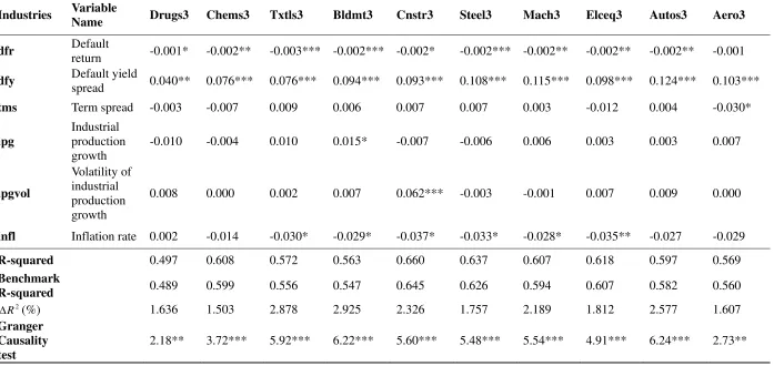
Many more clues of different effects can be found in the results (Table 7) under

the disaggregated classification of 40 industries, which is an extension of the

10-industry classification. A majority of the industries remain sensitive to the default

return and default yield spread. However, some sectors, such as Medeq3 (Medical

Equipment), Hardw3 (Computers), and Whlsl3 (Wholesale), react weakly to default

return surprises. Since these industries have longer profit cycles and the former two

industries require large initial investments, they may not be sensitive to the changes

in risk denoted by changes in realised bond return. Moreover, the insensitivity of

some industries to default return changes is mainly due to their small shares in the

stock market. These industries include Beer3 (Beer and Liquor), Aero3 (Aircraft),

and Chips3 (Electronic Equipment). The default yield remains significant among all

industries, except Smoke3 (Tobacco Products).

The differences of the impact of the four other factors are barely reflected in the

disaggregated classification. Cnstr3 (Construction), Bldmt3 (Construction Materials)

and Util3 (Utilities) are all cyclical industrial sectors that rely on raw materials and

heavy equipment. They are expected to be strongly influenced by output shocks,

which are shown in the coefficients for industrial production-related factors. Medeq3

(Medical Equipment), Cnstr3 (Construction), Bldmt3 (Construction Materials), and

Rlest3 (Real Estate) are greatly affected by inflation shocks. A possible explanation

is that these industries normally involve large start-up costs and high proportions of

physical capital.

Meanwhile, the Granger causality null hypothesis cannot be rejected for Hardw3

(Computers). It shows little increase in R-squared (0.87%) from the benchmark

(18)

forecast the subsequent volatility of stock returns in the computer industry.

The explanatory power of the predictive model (0.176) is higher than that of the

benchmark model (0.141) for Medeq3 (Medical Equipment). The relative increase of

R-squared is quite large (24.823%). This implies that the present volatility of Medeq3

(Medical Equipment) stock return depends weakly on the previous volatility, which is

consistent with its weak persistency (



10.2574,



2 0.2407). Nevertheless, this

industry is fairly sensitive to the default yield (0.171) and inflation rate (-0.087). This

indicates that the high-risk medical equipment industry fluctuates greatly with the

risk premium depending on the company’s quality (default yield) and price levels

(inflation rate).

Other industries with a relatively greater increase in R-squared include Bussv3

(Business Services), Hshld3 (Consumer Goods) and Clths3 (Apparel), where the last

two are also included in Nodur2 and Cnsmr1.

In summary, the impact of macroeconomic variables on stock return volatility is

largely consistent within a general industry classification, where macroeconomic

factors that cause volatility have significant effects, including default return and

default yield spread, while other factors do not. However, the differences in impact

are obvious within disaggregated sectors (10- and 40-industry classifications). For

example, the consumption-related and medical equipment industries show better

forecasts after these macroeconomic determinants are added to the benchmark

(19)

5. Out-of-Sample Analysis

5.1 Methodology

The target models in this section are the forecasting regressions in Equation (4),

while the macroeconomic variables contained in X_t₁ are different among

industries. Only those found to have a significant effect on industry stock return

volatility are included in the forecasting models.

The benchmark models have two specifications. One is the benchmark model in

Equation (5) and the other is the new model. The new model adds default return and

default yield to the right-hand side of the regression in Equation (5). These two

factors have obvious impacts on the stock return volatility of the whole market.

Specifically, the models are expressed as

Model 1 (benchmark model 1):

6

, , , ,

1

j t j j i j t i j t i

SRV





SRV  u



 



 , (6)

Model 2 (benchmark model 2):

6

, , , 1 1 ,

1

j t j j i j t i j t j t j t i

SRV





SRV _



dfr_



dfy_ u



 



   , (7)

Model 3 (new forecasting model):

6

, , , 1 ,

1

j t j j i j t i t j t i

SRV





SRV

_



X

_















. (8)

where Xt1 varies among industries, incorporating factors other than default return

and default yield, based on the results in Section 4.

Under the null hypothesis, the additional parameters in the new model cannot

predict the absence of Granger causality. The benchmark and alternative models

(20)

valid inferences are constructed under the conditions of asymptotic standard

normality. However, the conditions are violated because the models are nested. It is

recommended that the tests are adjusted because of the noise associated with the

larger model’s forecast (Clark and West, 2007). Thus, one-step-ahead forecasts are

used, and the sample MSPEs for the two models are given by

, ≡ ∑ , , , , , ≡ ∑ , , , , (9)

, ∑ , , , ∑ , ,

, , . (10)

The new forecasting model has a smaller MSPE than the benchmark model.

Clark and West (2007) propose testing the null hypothesis with

2 2

,1 ,2

ˆj (ˆj adjustmenti)

    instead of 2 2

,1 ,2

ˆ_j ˆ_j

  , rejecting the null hypothesis that the

test statistic is significantly positive. To simplify, the term is defined as

∑ , , , ∑ , , , ∑ , ,

, , . (11)

Hence, 2 2

,1 ,2

ˆ_j (ˆ_j adjustment_i)

    is the sample average of fˆ_t_₁ . The test

procedure for equal MSPE is to regress fˆ_t₁ on a constant and use the resulting

t-statistics for the zero coefficient test. The null is rejected if the statistic is bigger

than 1.282 (for a one-sided test under the 10% significance level), 1.645 (for a

one-sided test under the 5% significance level), or 2.326 (for a one-sided test under

(21)

In this paper, the Clark and West (2007) test is conducted on two groups of

models, on Model 1 and Model 3, and on Model 2 and Model 3, respectively. The

test examines whether the target forecasting models achieve higher predictive

accuracy over industries of different sorts than the benchmark models do.

Forecasting models are analysed through a rolling or recursive process within a

regression window of 20 years (240 months). The results in several periods are

reported, including those in the periods from 1947 to 2012, 1972 to 2012, 1982 to

2012, and 1972 to 2002. Since the forecasting performance is affected by the 1973 -

1975 oil shock (Welch and Goyal, 2008), the sample is split in the 1970s in order to

test the sensitivity of the results to the inclusion of the 1970s data.

5.2 Results

Tables 8a to 8d report the out-of-sample results for selected industries, using

rolling and recursive estimations. In each table, the format of the benchmark models

and new forecasting model, as well as the Clark and West (2007) test statistics

(multiplied by one million) and their significance levels are presented according to

industries. The Clark and West (2007) test results largely affirm the in-sample

findings – that the new forecasting models which including macroeconomic variables

improve predictive accuracy, when compared to the benchmark models of the AR (6)

process. This finding indicates that these macroeconomic variables Granger-cause

industry stock return volatility out of sample.

The upper panel of each table shows the Clark and West (2007) test results for

the comparison between the AR (6) benchmark model and the new forecasting model.

(22)

macroeconomic factors, outperform the AR (6) benchmark models. In particular, for

Manuf2 (Manufacturing, etc.), Fin3 (Trading) and Rlest3 (Real Estate), the null

hypothesis is rejected in a rolling or recursive estimation for most out-of-sample

periods. Meanwhile, some other industries, such as Medeq3 (Medical Equipment),

Cnstr3 (Construction) and Utils2 (Utilities), have better performance in the new

forecasting models.

The results in Tables 8s to 8d reveal that most new forecasting models improve

the predictive accuracy after the macroeconomic variables are changed. Based on the

results in Section 4.1, Manuf2 (Manufacturing, etc.), Hardw3 (Computers), Fin3

(Trading), and Rlest3 (Real Estate) all show convincing evidence that the modified

models predict better. Other industries, such as Cnstr3 (Construction), show

improvements only in the recursive estimations in the two sub-periods (1972–2012

and 1982–2012). The results show that the forecasts incorporating AR (6), default

return, default yield, volatility of industrial production growth and inflation are

relatively more accurate during the periods.

A comparison of results from the 1972 - 2002 and 1982 - 2012 periods

demonstrates that the predictive power for stock return volatility is sensitive to the

inclusion of the 1970s. For instance, the volatility of Manuf2 (Manufacturing, etc.)

seems to have better prediction with AR (6) and the default yield in the 1982 - 2012

period, using both rolling and recursive approaches. However, the same phenomenon

cannot be found during the 1972 - 2002 period.

The discrepancy between results obtained from the rolling and recursive

approaches is substantial. Generally, under a recursive scheme, the benchmark

(23)

new forecasting models. Nevertheless, in some cases, the results under the rolling

estimation display more significant model differences. For example, the augmented

model of Fin3 (Trading) industry outperforms the AR (6) regressions in the same

periods, except for the recursive scheme during the 1972 - 2012 and 1972 - 2002

periods, which cover the turbulent times during the 1970s. Meanwhile, the

augmented models improve the reliability of predictions in each sub-period, by

adding the factors of industrial production growth and inflation rate only under the

recursive scheme. Under the rolling estimation, the forecast sample is limited to 240

months (20 years) of data throughout the whole sample period, while under the

recursive scheme, the forecast sample grows continually one step ahead. Hence, the

forecasts under the recursive scheme might become less volatile and superior in the

out-of-sample performance as the sample size increases. This intuition is pronounced

in many industries, including Utils2 (Utilities), Medeq3 (Medical Equipment) and

Cnstr3 (Construction). Such prominence could be due to the greater volatility of

stock return in those industries.

6. Conclusion

Stock return volatility is largely countercyclical and is often connected to

macroeconomic determinants. This paper employs an augmented model to detect the

impacts of macroeconomic factors on stock return volatility in different industries.

The results show that the difference in the impacts of macroeconomic factors is

obvious among disaggregated industry sectors. Different levels of sensitivity of

industry-level stock return volatility are found in variables related to general

(24)

test is employed to verify whether the new forecasting models, which vary among

industries based on the in-sample results, can have better predictions than the two

benchmark models. Our results show that default return and default yield have

significant impacts on stock return volatility. The discrepancies of the influence

among disaggregated industries are conspicuous. For example, the Cnstr3

(Construction), Bldmt3 (Construction Materials) and Util3 (Utilities), which are all

cyclical industrial sectors that rely on raw materials and heavy equipment, are

strongly influenced by industrial production-related factors. Meanwhile, Medeq3

(Medical Equipment), Cnstr3 (Construction), Bldmt3 (Construction Materials), and

Rlest3 (Real Estate) are largely affected by inflation shocks.

As for the out-of-sample analysis, the new forecasting models perform better

than the benchmark models constructed by auto-regressions or basic settings for the

aggregate market. However, the superiority is not exactly the same under the two

approaches in four sub-periods.

This paper extends the results of previous studies mainly by Paye (2012) via

focusing on the industry-level analysis. The investigation proves that the impacts of

the examined macroeconomic factors differentiate themselves from one industry to

another. Furthermore, to some degree, the modified models improve the predictive

accuracy. The next intriguing step for future studies is to explore the specific reasons

(25)

References

Anderson, T. G., Bollerslev, T., and Diebold, F. X., 2007. Roughing it up: Including

jump components in the measurement, modelling, and forecasting of return

volatility. Review of Economics and Statistics 89(4), 701-720.

Boudoukh, J., Richardson, M., and Whitelaw, R. F., 1994. Industry returns and the

fisher effect. Journal of Finance 49(5), 1595-1615.

Campbell, J. Y., Lettau, M., Malkiel, B. G., and Xu, Y., 2001. Have individual stocks

become more volatile? An empirical exploration of idiosyncratic risk.

Journal of Finance 56(1), 1-43.

Chen, N. F., Roll, R., and Ross, S. A. 1986. Economic forces and the stock market.

Journal of Business 59(3), 383-403.

Clark , T. E., and West, K. D., 2007. Approximately normal tests for equal predictive

accuracy in nested models. Journal of Econometrics 138(1), 291-311.

Czaja , M. G., and Scholz, H., 2007. Sensitivity of stock returns to changes in the

term structure of interest rates—evidence from the German market. Operations

Research Proceedings 2006, 305-310.

Dinenis, E., and Staikouras, S. K., 1998. Interest rate changes and common stock

returns of financial institutions: evidence from the UK. European Journal of

Finance 4(2), 113-127.

Engle, R. F, Gyhsels, E., and Sohn, B., 2008. On the economic sources of

stock market volatility. AFA 2008 New Orleans Meetings Paper.

Engle, R. F., and Rangel, J. G., 2008. The spline-GARCH model for low-frequency

volatility and its global macroeconomic causes. Review of Financial Studies

21(3), 1187-1222.

(26)

market. Journal of Energy Finance and Development 4(1), 69-87.

Fama, E. F., and French, K. R., 1997. Industry costs of equity. Journal of Financial

Economics 43(2), 153-193.

Fornari, F., and Mele, A., 2013. Financial volatility and economic activity. Journal of

Financial Management, Markets and Institutions 2, 155-198.

Hess, M. K., 2003. Sector specific impacts of macroeconomic fundamentals on the

Swiss stock market. Financial Markets and Portfolio Management 17(2),

234-245.

Humpe, A., and Macmillan, P., 2009. Can macroeconomic variables explain

long-term stock market movements? A comparison of the US and Japan. Applied

Financial Economics 19(2), 111-119.

Kearney, C., and Daly, K., 1998. The causes of stock market volatility in Australia.

Applied Financial Economics 8(6), 597-605.

Merton, R. C., 1980. On estimating the expected return on the market: an exploratory

investigation. Journal of Financial Economics 8(4), 323-361.

Oertmann, P., Rendu, C., and Zimmermann, H., 2000. Interest rate risk of European

financial corporations. European Financial Management 6(4), 459-478.

Paye, B. S., 2012. ‘Déjà vol’: Predictive regressions for aggregate stock market

volatility using macroeconomic variables. Journal of Financial Economics

106(3), 527-546.

Sadorsky, P., 2001. Risk factors in stock returns of Canadian oil and gas companies.

Energy Economics 23(1), 17-28.

Sadorsky, P., 2003. The macroeconomic determinants of technology stock price

volatility. Review of Financial Economics 12(2), 191-205.

(27)

Journal of Finance 44(5), 1115-1153.

Sohn, B., 2009. Cross-section of equity returns: stock market volatility and priced

factors. Working Paper, Georgetown University.

Sweeney, R. J., and Warga, A. D., 1986. The pricing of interest-rate risk: evidence

from the stock market. Journal of Finance 41(2), 393-410.

Welch, I., and Goyal, A., 2008. A comprehensive look at the empirical performance

(28)

Stock Return Volatility of S&P 500 Value-weighted Market Portfolio

Stock Return Volatility of Manuf1 (manufacturing, energy and utilities)

Stock Return Volatility of Hitec1 (business equipment, telephone and television transmission)

Stock Return Volatility of S&P 500 Value-weighted Market Portfolio and Cnstr3 (construction)

[image:28.612.134.524.88.499.2]

Figure 1: Fluctuations of Stock Return Volatility (Range: 192701-201212)

0 .0 2 .0 4 .06

1930m1 1940m1 1950m1 1960m1 1970m1 1980m1 1990m1 2000m1 2010m1

Stock return volatility of S&P 500 value-weighted market portfolio Recession

0 .0 2 .0 4 .0 6

1930m1 1940m1 1950m1 1960m1 1970m1 1980m1 1990m1 2000m1 2010m1 Manuf1 Recession 0 .0 2 .0 4 .0 6

1930m1 1940m1 1950m1 1960m1 1970m1 1980m1 1990m1 2000m1 2010m1 HiTec1 Recession 0 .02 .0 4 .0 6 .08

1930m1 1940m1 1950m1 1960m1 1970m1 1980m1 1990m1 2000m1 2010m1

(29)

28

[image:29.792.72.719.180.420.2]

Table 1: Macroeconomic Variables: Descriptive Statistics (Range: 192701-201212)

Table 1 presents the descriptive statistics for the macroeconomic variables over the period 1927 - 2012. The Phillips and Perron unit root test is conducted for all macroeconomic variables. The final two columns report the test statistics for the Phillips and Perron unit root test and the associated Mackinnon approximate p-value, respectively. As shown, the test results reject the null hypothesis of a unit root for all variables, implying that persistence is not severe.

Phillips and Perron test

Symbol Variable Name Mean Std. Dev. Min Max p-value

dfr Default Return -0.0050 0.2137 -1.2854 2.6677 -37.04 0.00

dfy Default Yield 0.0180 0.0097 0.0035 0.0759 -3.99 0.00

tms Term Spread 0.0168 0.0132 -0.0365 0.0455 -4.77 0.00

ipg Industrial production growth 0.0026 0.0182 -0.1096 0.1532 -17.29 0.00

ipgvol Industrial Production Growth

Volatility 0.0090 0.0117 0.0000 0.1278 -21.52 0.00

(30)

29

[image:30.792.140.623.163.412.2]

Table 2: Stock Return Volatility: Industry Classifications and Descriptive Statistics

Industry Mean Std. Dev. Definition

Cnsmr1 0.0086 0.0054 Consumer Durables, Nondurables, Wholesale, Retail, and Some Services

(Laundries, Repair Shops)

Manuf1 0.0089 0.0063 Manufacturing, Energy, and Utilities

Hitec1 0.0099 0.0067 Business Equipment, Telephone and Television Transmission

Hlth1 0.0093 0.0057 Healthcare, Medical Equipment, and Drugs

Other1 0.0098 0.0072 Other -- Mines, Construction, Building Materials, Transportation, Hotels,

Bus Services, Entertainment, Finance

(31)

30

Industry Mean Std. Dev. Definition

Nodur2 0.0072 0.0047 Consumer Nondurables -- Food, Tobacco, Textiles, Apparel, Leather, Toys

Durbl2 0.0128 0.0081 Consumer Durables -- Cars, TV's, Furniture, Household Appliances

Manuf2 0.0097 0.0067 Manufacturing -- Machinery, Trucks, Planes, Chemicals, Off Furn, Paper,

Com Printing

Enrgy2 0.0108 0.0066 Oil, Gas, and Coal Extraction and Products

Hitec2 0.0126 0.0081 Business Equipment -- Computers, Software, and Electronic Equipment

Telcm2 0.0085 0.0060 Telephone and Television Transmission

Shops2 0.0091 0.0059 Wholesale, Retail, and Some Services (Laundries, Repair Shops)

Hlth2 0.0093 0.0057 Healthcare, Medical Equipment, and Drugs

Utils2 0.0079 0.0071 Utilities

Other2 0.0098 0.0072 Other -- Mines, Construction, Building Materials, Transportation, Hotels,

Bus Services, Entertainment, Finance

(32)

31

Bldmt3 0.0102 0.0070 Construction Materials

Cnstr3 0.0164 0.0110 Construction

Steel3 0.0133 0.0098 Steel Works Etc.

Industry Mean Std. Dev. Definition

Agric3 0.0130 0.0075 Agriculture

Food3 0.0075 0.0051 Food Products

Beer3 0.0119 0.0082 Beer & Liquor

Smoke3 0.0104 0.0062 Tobacco Products

Toys3 0.0171 0.0120 Recreation

Fun3 0.0150 0.0098 Entertainment

Books3 0.0125 0.0082 Printing and Publishing

Hshld3 0.0098 0.0063 Consumer Goods

Clths3 0.0095 0.0062 Apparel

Medeq3 0.0125 0.0097 Medical Equipment

Drugs3 0.0097 0.0059 Pharmaceutical Products

Chems3 0.0106 0.0072 Chemicals

(33)

32

Mach3 0.0110 0.0080 Machinery

Elceq3 0.0132 0.0084 Electrical Equipment

Autos3 0.0133 0.0083 Automobiles and Trucks

Aero3 0.0147 0.0097 Aircraft

Ships3 0.0131 0.0072 Shipbuilding, Railroad Equipment

Mines3 0.0127 0.0087 Non-Metallic and Industrial Metal Mining

Coal3 0.0169 0.0130 Coal

Oil3 0.0109 0.0066 Petroleum and Natural Gas

Util3 0.0079 0.0071 Utilities

Telcm3 0.0085 0.0060 Communication

Industry Mean Std. Dev. Definition

Bussv3 0.0120 0.0144 Business Services

Hardw3 0.0132 0.0082 Computers

(34)

33

Labeq3 0.0126 0.0071 Measuring and Control Equipment

Boxes3 0.0109 0.0062 Shipping Containers

Trans3 0.0114 0.0071 Transportation

Whlsl3 0.0117 0.0105 Wholesale

Rtail3 0.0095 0.0062 Retail

Meals3 0.0118 0.0065 Restaurants, Hotels, Motels

Banks3 0.0114 0.0093 Banking

Insur3 0.0111 0.0078 Insurance

Rlest3 0.0163 0.0131 Real Estate

Fin3 0.0122 0.0097 Trading

Other3 0.0126 0.0079 Almost Nothing

(35)

34

[image:35.792.60.737.187.395.2]

Table 3: Stock Return Volatility: Descriptive Statistics in Sub-periods (Five Industries) Stock

Return Volatility

1927-1955 1956-1984 1985-2012

Industry Mean Std. Dev. Max Min Mean Std. Dev. Max Min Mean Std. Dev. Max Min

Cnsmr1 0.0096 0.0069 0.0459 0.0025 0.0070 0.0030 0.0196 0.0023 0.0093 0.0051 0.0514 0.0030

Manuf1 0.0107 0.0078 0.0485 0.0028 0.0068 0.0032 0.0216 0.0015 0.0093 0.0064 0.0629 0.0027

Hitec1 0.0092 0.0074 0.0555 0.0021 0.0082 0.0035 0.0273 0.0027 0.0125 0.0076 0.0539 0.0046

Hlth1 0.0093 0.0072 0.0495 0.0027 0.0082 0.0037 0.0277 0.0025 0.0105 0.0054 0.0542 0.0030

Other1 0.0115 0.0084 0.0508 0.0029 0.0071 0.0032 0.0258 0.0023 0.0109 0.0080 0.0556 0.0029

S&P_vwv 0.0112 0.0082 0.0471 0.0027 0.0071 0.0032 0.0223 0.0019 0.0100 0.0062 0.0550 0.0031

Table 3 reports the stock return volatility of the aggregate market (S&P_vwv) and the industries based on the 5-industry classification in three sub-periods. The first period, 1927 - 1955, covers the Great Depression, while the last period, 1985 - 2012, features the Great Moderation and the 2008 global financial crisis.

(36)

35

[image:36.792.63.768.241.351.2]

Table 4: Correlation Coefficients

S&P_vwv dfr Dfy tms ipg ipgvol infl

S&P_vwv 1

Dfr -0.0566 1

Dfy 0.6574 -0.0198 1

Tms 0.1953 0.0746 0.2689 1

Ipg -0.1481 0.0912 -0.1363 0.0198 1

Ipgvol 0.2935 0.0305 0.2458 0.0522 0.0469 1

Infl -0.1491 0.0721 -0.1797 -0.0435 0.2726 -0.0047 1

Table 4 reflects the correlation coefficients between each two variables.

(37)

36

[image:37.792.70.728.162.445.2]

Table 5: In-sample Predictive Regression Results for 5-industry Classification

Symbol Variable Name S&P_vwv Cnsmr1 Manuf1 Hitec1 Hlth1 Other1

Dfr Default return -0.001* -0.001** -0.001* -0.001* -0.001** -0.002**

Dfy Default yield spread 0.088*** 0.080*** 0.083*** 0.053*** 0.046** 0.077***

Tms Term spread -0.002 -0.001 -0.002 -0.014 -0.002 0.000

Ipg Industrial production

growth -0.001 0.000 -0.001 0.002 -0.009 0.009

Ipgvol Volatility of industrial

production growth 0.006 0.004 0.012 -0.011 0.007 -0.004

Infl Inflation rate -0.015 -0.001 -0.012 -0.015 -0.005 -0.022

R-squared 0.584 0.494 0.563 0.607 0.475 0.616

Benchmark

R-squared 0.575 0.481 0.553 0.602 0.466 0.607

2

R

 (%) 1.565 2.703 1.808 0.831 1.931 1.483

Granger

Causality test 4.00*** 4.17*** 3.74*** 2.46** 2.47** 3.92***

(38)

37

[image:38.792.68.731.147.516.2]

Industries Variable

Name Nodur2 Durbl2 Manuf2 Enrgy2 Hitec2 Telcm2 Shops2 Hlth2 Utils2 Other2

dfr Default

return -0.002*** -0.002** -0.001 -0.002** -0.001* -0.001** -0.002** -0.001** -0.001* -0.002**

dfy Default yield

spread 0.056*** 0.121*** 0.095*** 0.065*** 0.077*** 0.051*** 0.070*** 0.046** 0.084*** 0.077***

tms Term spread 0.002 0.003 -0.002 -0.003 -0.023* -0.003 -0.003 -0.002 -0.009 0.000

ipg

Industrial production growth

0.000 0.003 0.001 -0.001 0.003 -0.002 -0.004 -0.009 -0.003 0.009

ipgvol

Volatility of industrial production growth

-0.007 0.013 0.011 -0.002 -0.009 -0.006 -0.002 0.007 0.022* -0.004

infl Inflation rate -0.003 -0.023 -0.018 -0.010 -0.024 -0.005 0.002 -0.005 -0.010 -0.022

R-squared 0.463 0.596 0.570 0.528 0.609 0.550 0.550 0.475 0.642 0.616

Benchmark

R-squared 0.452 0.582 0.559 0.522 0.602 0.544 0.540 0.466 0.633 0.607

2

R

 (%) 2.434 2.405 1.968 1.149 1.163 1.103 1.852 1.931 1.422 1.483

Granger Causality test

(39)

38

[image:39.792.52.750.151.492.2]

Industries Variable

Name Agric3 Food3 Beer3 Smoke3 Toys3 Fun3 Books3 Hshld3 Clths3 Medeq3

dfr Default return -0.002*** -0.002*** -0.001 -0.002*** -0.003*** -0.002* -0.002*** -0.002*** -0.004** -0.002

spread 0.065*** 0.067*** 0.072*** 0.016 0.154*** 0.165*** 0.076*** 0.082*** 0.064*** 0.171***

tms Term spread -0.017 0.000 -0.009 0.000 -0.019 -0.010 0.006 -0.019 0.003 -0.003

ipg

-0.004 0.002 0.020** -0.007 0.005 0.005 0.033*** 0.006 -0.003 -0.002

ipgvol

-0.002 -0.007 0.022 -0.018 0.057*** 0.014 0.012 0.000 -0.001 0.041

infl Inflation rate -0.018 -0.006 -0.007 -0.001 -0.020 -0.005 -0.029 -0.010 -0.008 -0.087***

R-squared 0.530 0.488 0.604 0.517 0.625 0.591 0.544 0.461 0.503 0.176

Benchmark

R-squared 0.519 0.474 0.597 0.512 0.610 0.579 0.529 0.445 0.478 0.141

2

R

 (%) 2.119 2.954 1.173 0.977 2.459 2.073 2.836 3.596 5.230 24.823

4.02*** 4.52*** 2.72** 2.30** 6.67*** 5.14*** 5.32*** 4.99*** 7.62*** 7.09***

(40)

39

[image:40.792.53.750.152.482.2]

Table 7: In-sample Predictive Regression Results for 40-industry Classification (Continued)

Name Drugs3 Chems3 Txtls3 Bldmt3 Cnstr3 Steel3 Mach3 Elceq3 Autos3 Aero3

dfr Default

return -0.001* -0.002** -0.003*** -0.002*** -0.002* -0.002*** -0.002** -0.002** -0.002** -0.001

spread 0.040** 0.076*** 0.076*** 0.094*** 0.093*** 0.108*** 0.115*** 0.098*** 0.124*** 0.103***

tms Term spread -0.003 -0.007 0.009 0.006 0.007 0.007 0.003 -0.012 0.004 -0.030*

ipg

-0.010 -0.004 0.010 0.015* -0.007 -0.006 0.006 0.003 0.003 0.007

ipgvol

0.008 0.000 0.002 0.007 0.062*** -0.003 -0.001 0.007 0.009 0.000

infl Inflation rate 0.002 -0.014 -0.030* -0.029* -0.037* -0.033* -0.028* -0.035** -0.027 -0.029

R-squared 0.497 0.608 0.572 0.563 0.660 0.637 0.607 0.618 0.597 0.569

Benchmark

R-squared 0.489 0.599 0.556 0.547 0.645 0.626 0.594 0.607 0.582 0.560

2

R

 (%) 1.636 1.503 2.878 2.925 2.326 1.757 2.189 1.812 2.577 1.607

(41)

40

[image:41.792.49.748.159.515.2]

Name Ships3 Mines3 Coal3 Oil3 Util3 Telcm3 Bussv3 Hardw3 Chips3 Labeq3

dfr Default

return -0.001 -0.001* -0.004** -0.002** -0.001* -0.001** -0.002 -0.001 -0.001 -0.002***

spread 0.118*** 0.065** 0.174*** 0.069*** 0.083*** 0.051*** 0.276*** 0.044** 0.067** 0.071***

tms Term spread 0.011 -0.014 0.002 -0.005 -0.009 -0.003 -0.026 -0.027** -0.024 -0.014

ipg

0.003 0.012 0.011 0.000 -0.003 -0.002 -0.086*** 0.003 0.005 -0.013

ipgvol

0.004 -0.014 0.004 -0.005 0.022* -0.006 0.064* -0.017 0.015 -0.012

infl Inflation rate -0.013 -0.025 -0.008 -0.011 -0.010 -0.005 -0.006 -0.016 -0.032 -0.012

R-squared 0.542 0.569 0.503 0.538 0.644 0.550 0.275 0.580 0.563 0.555

Benchmark

R-squared 0.529 0.563 0.489 0.531 0.635 0.544 0.236 0.575 0.554 0.541

2

R

 (%) 2.457 1.066 2.863 1.318 1.417 1.103 16.525 0.870 1.625 2.588

(42)

41

[image:42.792.49.754.145.510.2]

Name Boxes3 Trans3 Whlsl3 Rtail3 Meals3 Banks3 Insur3 Rlest3 Fin3 Other3

dfr Default

return -0.001** -0.002** 0.000 -0.002*** -0.001 -0.002*** -0.001 -0.004*** -0.002** -0.002**

spread 0.079*** 0.111*** 0.171*** 0.059*** 0.084*** 0.071*** 0.096*** 0.118*** 0.066** 0.084***

tms Term spread -0.004 0.000 -0.019 -0.003 -0.021* -0.017 -0.019 0.000 -0.022 -0.018

ipg

-0.005 -0.002 0.036*** -0.005 0.008 0.007 -0.005 0.021 0.026** 0.015

ipgvol

-0.011 0.000 0.019 -0.004 0.004 0.012 -0.009 0.030 -0.018 0.019

infl Inflation rate -0.005 -0.006 -0.014 0.003 -0.013 -0.036** -0.022 -0.080*** -0.050*** -0.024

R-squared 0.507 0.583 0.489 0.564 0.514 0.692 0.576 0.669 0.620 0.551

Benchmark

R-squared 0.495 0.571 0.479 0.555 0.504 0.681 0.563 0.654 0.609 0.538

2

R

 (%) 2.424 2.102 2.088 1.622 1.984 1.615 2.309 2.294 1.806 2.416

(43)

[image:43.612.126.527.81.355.2]

Table 8a: Out-of-sample Test Results for Predictive Accuracy

Manuf2 1947m1-2012

m12 1972m1-2012 m12 1982m1-2012 m12 1972m1-2002 m12 Benchmark

model AR(6) AR(6) AR(6) AR(6)

New model +dfy +dfy +dfy +dfy

Rolling

estimation 4.04** 2.70 3.50 0.41

Recursive

estimation 6.61*** 2.42* 5.97*** 0.94

1947m1-2012 m12 1972m1-2012 m12 1982m1-2012 m12 1972m1-2002 m12 Benchmark

model +dfr, dfy +dfr, dfy +dfr, dfy +dfr, dfy

Rolling

estimation 8.82* 13.90* 18.10* -0.04

Recursive

estimation 0.13 0.12 0.01 0.16

Utils2 1947m1-2012

model AR(6) AR(6) AR(6) AR(6)

Rolling

estimation -1.02 -4.49 -5.66 -0.80

Recursive

estimation 2.09* -0.91 1.70 -1.51

1947m1-2012 m12 1972m1-2012 m12 1982m1-2012 m12 1972m1-2002 m12 Benchmark

Rolling

estimation 6.96 10.40 13.90 -0.68

Recursive

estimation 1.25 0.84 0.48 0.43*

(44)

[image:44.612.128.527.82.355.2]

Table 8b: Out-of-sample Test Results for Predictive Accuracy (continued)

Medeq3 1947m1-2012

model AR(6) AR(6) AR(6) AR(6)

New model +dfy, infl, dfr +dfy, infl, dfr +dfy, infl, dfr +dfy, infl, dfr

Rolling

estimation 18.60*** 4.95 7.48 -1.67

Recursive

estimation 32.70*** 5.73 24.00** -12.50

New model +dfy, infl, dfr +dfy, infl, dfr +dfy, infl, dfr +dfy, infl, dfr

Rolling

estimation 1.20 0.10 1.27 -1.89

Recursive

estimation 5.79** 5.12 6.59* -1.84

Cnstr3 1947m1-2012

model AR(6) AR(6) AR(6) AR(6)

New model +dfr, dfy,

ipgvol, infl +dfr, dfy, ipgvol, infl +dfr, dfy, ipgvol, infl +dfr, dfy, ipgvol, infl Rolling

estimation 12.60 15.50 21.00 3.49

Recursive

estimation 9.02** 7.38 15.70** -3.59

New model +dfr, dfy,

ipgvol, infl +dfr, dfy, ipgvol, infl +dfr, dfy, ipgvol, infl +dfr, dfy, ipgvol, infl Rolling

estimation 3.93 6.18 7.38 2.62

Recursive

estimation 2.65 5.34* 6.64* -0.59

(45)

[image:45.612.128.527.82.355.2]

Table 8c: Out-of-sample Test Results for Predictive Accuracy (continued)

Hardw3 1947m1-2012

model AR(6) AR(6) AR(6) AR(6)

New model +dfr, dfy, tms +dfr, dfy, tms +dfr, dfy, tms +dfr, dfy, tms

Rolling

estimation 2.59 2.89 0.65 6.35*

Recursive

estimation 6.19** 2.97 0.18 4.28

New model +dfr, dfy, tms +dfr, dfy, tms +dfr, dfy, tms +dfr, dfy, tms

Rolling

estimation 4.26* 6.87* 4.75 6.44*

Recursive

estimation 3.85* 3.64 0.00 4.78

Fin3 1947m1-2012

model AR(6) AR(6) AR(6) AR(6)

New model +dfr, dfy, ipg,

infl

+dfr, dfy, ipg, infl

Rolling

estimation 18.1** 22.9* 30.4* 2.84**

Recursive

estimation 7.94*** 4.86 11.8** -4.42

New model +dfr, dfy, ipg,

infl

+dfr, dfy, ipg, infl

Rolling

estimation 0.73 0.44 0.42 -0.08

Recursive

estimation 3.08** 4.72* 5.11* 2.36**

(46)

[image:46.612.127.526.82.354.2]

Table 8d: Out-of-sample Test Results for Predictive Accuracy (continued)

Rlest3 1947m1-2012

m12

1972m1-2012 m12

1982m1-2012 m12

1972m1-2002 m12

Benchmark

model AR(6) AR(6) AR(6) AR(6)

New model +dfr, dfy, infl +dfr, dfy, infl +dfr, dfy, infl +dfr, dfy, infl

Rolling

estimation 82.60*** 39.60*** 52.20*** 16.20***

Recursive

estimation 139.00*** 128.00*** 126.00*** 86.80***

1947m1-2012 m12

1972m1-2012 m12

1982m1-2012 m12

1972m1-2002 m12

Benchmark

New model +dfr, dfy, infl +dfr, dfy, infl +dfr, dfy, infl +dfr, dfy, infl

Rolling

estimation 2.94 4.67 5.88 -0.46

Recursive

estimation 8.39*** 12.30*** 10.80** 6.94***