Munich Personal RePEc Archive
Refinement of the Equilibrium of Public
Goods Games over Networks: Efficiency
and Effort of Specialized Equilibria
Pandit, Parthe and Kulkarni, Ankur
Indian Institute of Technology Bombay
7 July 2016
Online at
https://mpra.ub.uni-muenchen.de/72425/
Refinement of the Equilibrium of Public Goods Games
over Networks: Efficiency and Effort of Specialized
Equilibria
Parthe Pandit
Ankur A. Kulkarni
∗Abstract
Recently Bramoulle and Kranton [2] presented a model for the provision of public goods over a network and showed the existence of a class of Nash equilibria called specialized equilibria wherein some agents exert maximum effort while other agents free ride. We examine the efficiency, effort and cost of special-ized equilibria in comparison to other equilibria. Our main results show that the welfare of a particular specialized equilibrium approaches the maximum welfare amongst all equilibria as the concavity of the benefit function tends to unity. For forest networks a similar result also holds as the concavity approaches zero. Moreover, without any such concavity conditions, there exists for any network a specialized equi-librium that requires the maximum weighted effort amongst all equilibria. When the network is a forest, a specialized equilibrium also incurs the minimum total cost amongst all equilibria. For well-covered forest networks we show that all welfare maximizing equilibria are specialized and all equilibria incur the same total cost. Thus we argue that specialized equilibria may be considered as a refinement of the equilibrium of the public goods game. We show several results on the structure and efficiency of equilibria that highlight the role of dependants in the network.
1
Introduction
Recently, Bramoulle and Kranton [2] introduced a model for studying the incentives of agents for the provision of non-excludable public goods in the presence of a network amongst the agents. In their model, agents benefit from their own effort and also from the collective effort of their neighbours in the network, according to a monotone concave benefit function. Since effort is costly, agents choose their effort levels based on the efforts by their neighbours. In fact, some agents may choose to free ride, i.e., exert no effort, if the cumulative effort of their neighbours is such that marginal cost of their effort is higher than its marginal benefit. At a Nash equilibrium [6] of the resulting game, no agent has an incentive to unilaterally deviate from its effort level. Such a model, as the authors describe, is suitable to study the incentives for companies to invest in innovation and research, in the presence of a network of companies.
Bramoulle and Kranton [2] considered three classes of equilibria. In a specialized equilibrium, some agents exert maximum effort (effort they would exert in the absence of a network) and all other agents free ride. Equilibria where all agents exert a positive effort are calleddistributed equilibriaand equilibria which are neither specialized nor distributed are referred to ashybrid equilibria. Bramoulle and Kranton showed that there may not exist an efficient equilibrium, i.e., a profile of efforts in equilibrium may not correspond to that which maximizes social welfare. Hence it is relevant to compare only equilibrium profiles based on their welfare and ask which equilibria yield maximum welfare.
Recall that for a class of games G the Nash equilibrium may be thought of as a set-valued function that prescribes a set of strategy profiles, NE(G), for each game in G ∈ G. A refinement of the Nash equilibrium is another set-valued function which prescribes for eachG∈ G a subset of strategy profiles,
R(G) ⊆ NE(G), with the property that, for any G ∈ G, R(G) is nonempty if NE(G) is nonempty, and that there is some G∈ G such thatR(G)6= NE(G). Refined equilibria have additional properties
∗Parthe and Ankur are with the Systems and Control Engineering group at the Indian Institute of
Tech-nology Bombay, Mumbai, India 400076. They can be contacted at [email protected] and
specified by the mappingRand may be regarded as being more attractive for consideration as a solution concept. Bramoulle and Kranton [2] showed that specialized equilibria always exist, and under certain conditions, they have the property of stability under best response dynamics and hence may be considered as a refinement of the Nash equilibrium of the public goods game. However, it is not clear how these equilibria rank under the criterion of maximum equilibrium welfare and whether they lead to maximum total equilibrium effort or minimum total equilibrium cost. More generally, it is of interest to understand how the nature of the network affects the structure and efficiency of equilibria of a public goods game.
The present paper is born out of the observation that answers to these questions are within reach from our previous work in graph theory [7]. It was shown in [2] that specialized equilibria are in a one-to-one correspondence with maximal independent sets of the network. While in [7], we provided new characterizations of the cardinality of thelargest and thesmallest maximal independent set in a graph. Building on this characterization, in this paper, we show that specialized equilibria may be considered as a refinement of the equilibrium of a public goods game under certain broad assumptions and criteria. Our first result shows that under certain assumptions on the concavity of the benefit function, there exist specialized equilibria which attain the maximum welfare amongst all equilibria. Specifically, there is a particular specialized equilibrium with the property that as the concavity approaches unity, the welfare under this equilibrium comes arbitrarily close to the maximum equilibrium welfare. If the graph is a forest, a similar result holds even as the concavity approaches zero. Moreover, for a class of networks called well-covered forests [8], we show that for any benefit function, all welfare maximizing equilibria are necessarily specialized. A well-covered forest is a graph without cycles and isolated vertices wherein every vertex is either adjacent to exactly one other vertex, or has exactly one neighbour that possesses this property.
Next, considering the total weightedeffort as the criterion for comparing equilibria, we show that for any benefit function, there exist specialized equilibria that maximize the total weighted effort amongst all equilibria. Hence specialized equilibria may be considered as a refinement of the equilibrium of a public goods game by the criterion of total weighted effort, and also by the criterion of welfare under certain assumptions on the concavity of the benefit function. Surprisingly, analogous results do not hold for the criterion of minimum total cost, or minimum total effort – in general hybrid or distributed equilibria may lead to the least total cost. In fact, in regular networks distributed equilibria form a refinement of the equilibrium under the criterion of minimum total cost. However, if the network is a forest, we find that there is a specialized equilibrium that attains the minimum total equilibrium cost. Once again, well-covered forest networks have an interesting property – all equilibria on such networks require the
same total effort.
Additionally, we derive results relating the nature of equilibria and their efficiency to the structure of the underlying network of agents. We have found that the absence of cycles (i.e., forest networks) and the presence of dependants, i.e., agents having only one neighbour, is an important characteristic of the network in this regard. These results may have sociological interpretations and may be of independent interest.
The following section introduces the model and formally states the main results of this paper.
1.1
Model, terminology and main results
Let the graphG = (V, E)be a network with agents represented by vertices V ={1, . . . , n}, and with linksErepresenting pairwise connectivity between the agents, be it geographical, economic or social [2]. We first recall some terminology pertaining to graphs. Two verticesi, j ∈V are said to beadjacent if there exists an link(i, j)∈Ebetween them. Adjacent agents are also calledneighbours. An independent set of a graph is a set of pairwise nonadjacent vertices. An independent set is said to bemaximal if it is not a subset of a larger independent set. An independent set with the largest number of vertices is called amaximum independent set. The cardinality of a maximum independent set is called theindependence number and is denoted by α(G). It is easy to see that a maximum independent set is maximal, but the converse is not true. A generalization of the independence number is the w-weighted independence number for a vector1
of weightsw= (w1, . . . , wn)⊤,wi≥0for alli∈V. Define the weight of a setS⊆V as P
i∈Swi. The w-weighted independence number αw(G)is the maximum weight among the weights of all independent sets, and the independent set with the maximum weight is called the w-weighted maximum independent set. Clearlyαe(G)is the independence number ofG, wheree:= (1,1, . . . ,1)⊤ is
the vector of all 1’s.
1
A path between vertices i and j is a collection of distinct links(y1, z1), . . . ,(yk, zk)such that y1 = i, zk =j and zt=yt+1 for all 1≤t < k. Recall that a graph is said to beconnected if there is a path
between every pair vertices. A path that starts and ends at the same vertex is called a cycle. A forest is a graph without cycles. A connected forest is called a tree.
We now come back to the model for the game. Let every agent i∈V exert an effort xi ≥0 with a constant marginal costc. We call the vectorx= (x1, x2, . . . , xn)⊤as theprofile of efforts. Letb:R→R be a differentiable concave monotone benefit function, i.e., b′(y) >0, b′′(y)< 0 for all y ∈ R, y ≥0.
Moreover let b′(e∗) = c, for some e∗ > 0. In the absence of the network, an agent benefits b(x
i) on exerting an effortxi, which costscxi, whereby the utility of agent iis Usolo
i =b(xi)−cxi. This utility is maximum for a unique effort level e∗, since b is an increasing concave function, which by definition,
satisfies ∂U
solo i
∂xi (e
∗) = 0.
Due to presence of the network, however, an agent i benefits from the collective efforts exerted by itself and its neighboursNi:={j|(i, j)∈E}. Hence the benefit of agentiis,
b
xi+ X j∈Ni
xj
=b(Ei(x)),
where,
Ei(x) :=xi+ X j∈Ni
xj, (1)
is theeffort of the closed neighbourhood of agent i. It is the cumulative effort from which agent i can benefit. Hence the utility of agenti is
Ui(x) =b(Ei(x))−cxi. (2)
A profile of effortsx∗is aNash equilibrium [6] if no agent has an incentive to deviate from it unilaterally,
i.e.,
Ui(x∗i, x∗(−i))≥Ui(xi, x∗(−i)), for allxi≥0,
where x∗
(−i)= (x∗1, . . . , x∗i−1, x∗i+1, . . . , x∗n)⊤. For a public goods game over a networkG, we denote by
NE(G)the set of Nash equilibrium effort profiles.
It was shown in [2], that for every Nash equilibriumx, we have0≤xi ≤e∗. An agentiis called afree
rider ifxi= 0and aspecialist ifxi=e∗. An equilibriumx∗is said to bespecialized ifx∗i = 0orx∗i =e∗ for all agentsi. x∗ is said to be distributed if x∗
i >0 for all agentsi. We denote the set of specialized equilibria bySNE(G)and the set of distributed equilibria byDNE(G). Bramoulle and Kranton [2] also showed that in any specialized equilibrium, the agents exerting effort e∗ form a maximal independent
set of the graph. Conversely, every maximal independent set corresponds to a specialized equilibrium in which the agents in the set exert efforte∗ and all other agents free ride.
Among all equilibria of a public goods game, some equilibria may be more efficient than others. Carrying forward the discussion by Bramoulle and Kranton, we use the utilitarian definition of welfare to compare efficiency of effort profiles. The utilitarian welfare, WU(x), is the sum of utilities of each
agent at the profile of effortsx= (x1, x2, . . . , xn)⊤,
WU(x) :=
X i∈V
Ui(x) = X i∈V
b(Ei(x))−c e⊤x. (3)
An effort profile xis said to be efficient ifWU(x)≥WU(y), for all other effort profilesy. It was shown
in [2] that Nash equilibria are in general not efficient.
We denote the maximum equilibrium welfare by W∗U. Similarly, for a vector of weights w ∈ Rn, E∗w denotes the maximum w-weighted equilibrium effort and C∗ the minimum equilibrium cost.
Cor-respondingly WS∗
U, E S∗
w C
S∗ are these optimum quantities if only specialized equilibria are considered.
Formally,
WU∗ = max{WU(x)|x∈NE(G)}, WUS∗= max{WU(x)|x∈SNE(G)}, (4) E∗w= max{w⊤x|x∈NE(G)}, EwS∗= max{w⊤x|x∈SNE(G)}, (5)
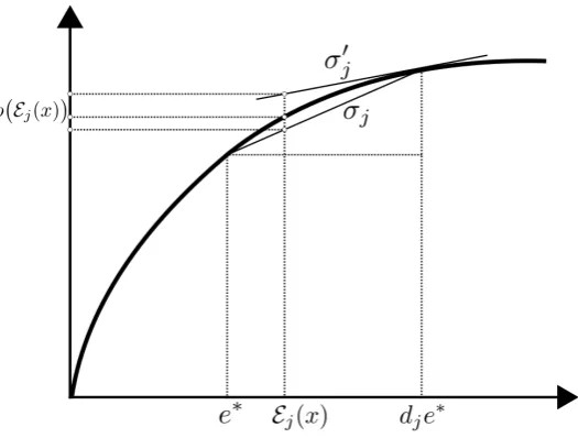
Figure 1: This figure (not to scale) describes the two extreme cases of concavity. Observe that as
σb→1, the benefit function is nearly linear in the interval[e∗, ne∗]and having slopeb′(e∗), whereas as
σb→0, the benefit function plateaus. Note however that asσb is varied,b(e∗)andb′(e∗)remains fixed whereby there is no scaling and hence equilibria remain unchanged.
The set of Nash equilibria which yield the maximum equilibrium welfare W∗U are called the welfare
maximizing equilibria, equilibria maximizing thew-weighted effort are calledeffort maximizing equilibria
and equilibria minimizing the cost are calledcost minimizing equilibria. Clearly, from equations (4 - 6), we have that,
W∗U≥WUS∗, E∗w≥ESw∗ and C∗≤CS∗. (7)
The problem of showing that specialized equilibria are a refinement insofar as maximum welfare is concerned amounts to showing the equalityW∗U=WUS∗. Similarly, to show that specialized equilibria are
a refinement with respect to maximum total weighted effort and minimum total cost we need to show thatE∗
w=E
S∗
w andC∗=C
S∗, respectively.
Notice that Ei(·) is a linear function of x and hence b(Ei(·)) is a concave function, whereby the objective functions in (4 - 6) are either concave or linear. However the feasible region NE(G) is non-convex and non-polyhedral andSNE(G)is an integer lattice (this follows from Theorem 7 later). Hence, showing that specialized equilibria are a refinement under any of the criteria above is a hard problem. Importantly, the non-polyhedrality of NE(G) implies that these claims cannot be arrived at using an argument based on extreme points or linear programming.
Let
σb:=
b(ne∗)−b(e∗)
ce∗(n−1) ,
denote the concavity of the benefit function b as defined by [2]. It is the normalized slope of the “secant” betweene∗ andne∗for the functionb. Sinceb is a strictly increasing function,σ
b>0, whereas since b is strictly concave, the slope of the secant is less than the slope of the tangent at e∗, whereby
cσb< b′(e∗) =c, i.e., σb<1.
In our analysis we consider two extreme cases, namely, asσb approaches unity and asσb approaches zero. While we varyσb,we assume that b′(e∗) =ccontinues to hold and b(e∗)remains unchanged with
σb. The two cases are depicted in Figure 1. Asσb →1, the slope of the secant tends to the slope of b ate∗. Since the function lies between the tangent and the secant, the function isnear-linear betweene∗
andne∗ asσ
b→1. On the other hand, as σb→0, the benefit functionplateaus beyonde∗. An important consequence of holding b(e∗) and b′(e∗) fixed is that it ensures that as σ
b changes, the Nash equilibria of the game do not change (see Lemma 7). This allows one to study the welfare of particular equilibria in comparison with W∗U with varying σb. Bramoulle and Kranton showed that as
σb→1the welfare function approaches the totald-weighted effort (plus a constant), wheredis a vector of degrees2
of agents. We show that asσb→0 the welfare function equals thenegative of the total cost (plus a constant). As a consequence, when σb → 1, the problem of equilibrium welfare maximization resembles the maximization of the totald-weighted equilibrium effort while asσb→0, it resembles the total equilibrium cost minimization.
Our first main result in this paper concerns these extreme regimes ofσb.
Theorem 1 (Welfare of specialized equilibria)
For a public goods game over a network without isolated agents,
(a) Let d= (d1, . . . , dn)⊤ be the vector of degrees of agents, i.e., di =|Ni| for all i∈ V.Let S∗ be a
maximum d-weighted independent set in the network and let x∗ be the specialized equilibrium with
agents inS∗as specialists and the rest as free riders. Then, asσ
b→1, the welfare ofx∗approaches
the maximum equilibrium welfare, i.e.,
lim
σb→1
WU∗ = lim
σb→1
WU(x∗) =n b(e∗)−ce∗+ce∗αd(G).
Consequently,limσb→1W
∗
U= limσb→1W S∗
U .
(b) Suppose the network is a forest. Let S′ be the smallest maximal independent set in the network
and let x′ be the specialized equilibrium with agents inS′ as specialists and the rest as free riders.
Then asσb→0, the welfare ofx′ approaches the maximum equilibrium welfare, i.e.,
lim
σb→0
W∗U= lim
σb→0
WU(x′) =nb(e∗)−ce∗β(G),
where β(G) is the size ofS′. Hence, for forests,lim
σb→0W
∗
U= limσb→0W S∗
U.
(c) The welfare of any distributed equilibrium (if it exists) is independent ofσb. Moreover,
WDU∗≥ lim
σb→0
WUS∗,
where,
WDU∗= inf{WU(x)|x∈DNE(G)},
is the least welfare attained by a distributed equilibrium.
The assumption regarding the absence of isolated agents does not cause loss of generality, and has been made here for the sake of simplicity. Isolated agents i derive benefits from their own efforts only and hence exert the same efforte∗ in any equilibrium. Hence their utility at an equilibriumxis always
Usolo
i (x) =b(e∗)−ce∗ which is independent of σb (sinceb(e∗)andb′(e∗)are fixed).
Notice that Theorem 1(a) is a general result pertaining to any network. Equivalently, it says that for any networkGandǫ >0, there exists a thresholdσH such that for all benefit functions with fixedb(e∗) andb′(e∗) =cand σ
b≥σH,
0≤W∗U−WU(x∗)≤ǫ.
Theorem 1(b) pertains specifically to forests (Theorem 1(a) applies to forests too). Here we have that for any forestGandǫ >0, there exists a thresholdσLsuch that for all benefit functions with fixedb(e∗) andb′(e∗) =cand σ
b≤σL,
0≤WU∗−WU(x′)≤ǫ.
In Theorem 1(c), notice thatWD∗
U is theleastwelfare over distributed equilibria. The above theorem is a
consequence of a more general result regarding the ranking of equilibria when they are compared based on their total weighted effort and total cost which are given by Theorem 2 below.
It is worth noting that in both Theorems 1 and 2, we not only show that there exists a specialized equilibrium, but also point to a particular equilibrium which approaches the maximum welfare amongst all equilibria, under the given conditions on the concavity or the structure of the network.
Theorem 2 (Total effort and cost of specialized equilibria)
For a public goods game over a network,
(a) Letw= (w1, . . . , wn)⊤, wi≥0for alli∈V, be a set of weights andS∗ be a maximumw-weighted
independent set. Then the specialized equilibrium in which agents inS∗ exert efforte∗and the rest
are free riders is an effort maximizing equilibrium. Consequently, E∗
w=E
S∗
w.
(b) Suppose the network is a forest, and letS′ be the smallest maximal independent set in the network.
Then the specialized equilibrium in which agents inS′ exert efforte∗ and the rest are free riders is
a cost minimizing equilibrium. Consequently, for forest networks, C∗=CS∗.
(c) If there exists a distributed equilibriumx= (x1, . . . , xn)⊤, the cost incurred in it,Picxi, is at most
as much as that of any specialized equilibrium, wherebyC∗≤CD∗≤CS∗, where CD∗ the minimum
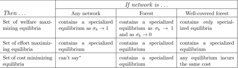
If network is
. . .
Then
. . .
Any network Forest Well-covered forestSet of welfare maxi-mizing equilibria
contains a specialized equilibrium asσb →1
contains a specialized equilibrium as σb → 1 and as σb →0
contains only special-ized equilibria
Set of effort maximiz-ing equilibria
contains a specialized equilibrium
contains a specialized equilibrium
contains a specialized equilibrium
Set of cost minimizing equilibria
can’t say∗ contains a specialized
equilibrium
any equilibrium incurs the same cost
Table 1: Summary of the main results in this paper – Theorems 1, 2 and 3.
∗If the network is regular then there always exists a distributed equilibrium where all agents exert equal
effort. This equilibrium minimizes the total cost.
(d) If the network is regular3
, a distributed equilibrium in which all agents exert equal effort minimizes the equilibrium cost, i.e., C∗=CD∗.
Notice that the above theorem does not require any assumptions about the benefit function.
We show that a particular class of networks called well-covered forests happen to have even stronger and more interesting properties. A networkGis said to bewell-covered if all maximal independent sets of Ghave the same size. For a network, if an agent i is adjacent to exactly one other agentj, we say thatiis adependant ofj, andj is theguardian ofi. It was shown by Plummer [8] that a forest network (without isolated agents) is well-covered if and only if all agents are either dependants or guardians, and every guardian agent has exactly one dependant. Our last main result is the following theorem regarding welfare maximizing equilibria in well-covered forest networks. Notice that this result holds without any assumptions on the benefit function orσb.
Theorem 3 (Efficient specialized equilibria in well-covered networks)
For a public goods game over a well-covered forest network,
(a) An equilibrium yields the maximum equilibrium welfare only if it is a specialized equilibrium.
(b) If the network does not have isolated agents, the cost incurred by any equilibrium profile of efforts is 1
2ce
∗n.
All our results are comprehensively summarized in Table 1.
Additionally, we obtain results that clarify the structure of equilibrium profiles in such games. In an equilibrium, if two neighbouring agentsi andj exert positive effortsxi and xj such that xi+xj =e∗, then we call such agentsco-specialists, and the link(i, j)joining them is called aco-specialist link. We show in Section 3 that, in any network at equilibrium, dependants are either specialists, or free riders, or that they form a co-specialist pair with their guardian. Interestingly, for networks with at least one dependant, we find that any Nash equilibrium has at least one free rider, i.e., there exists no distributed equilibrium. We further show that if the network is a forest, then at equilibrium, agents are either specialists, co-specialists or free riders only.
1.2
Organization of the paper
The rest of the paper is organised as follows. Section 2 provides some background on graphs and main results from our previous work in graph theory. In Section 3, we characterize the Nash equilibria in a public goods game over a network and discuss the effect of the network on the structure of the equilibrium. In particular, we discuss results about networks which havedependant andguardian agents. The proof of Theorem 2 is given in Section 4 which shows that specialized equilibria are a refinement under the criterion of maximum weighted equilibrium effort for all networks, while they are a refinement under the criterion of minimum equilibrium cost if the network is a forest. Section 5 proves Theorem 1 and shows that the specialized equilibrium is a refinement with respect to maximum equilibrium welfare under conditions on the concavity of the benefit function. In section 6, the result in Theorem 3 is proved
[image:7.595.73.529.72.202.2]which gives conditions on equilibria in a well-covered forest network for any benefit function. Finally, section 7 concludes the paper. In every case where the specialized equilibria form a refinement of the Nash equilibrium, we give the specialized equilibrium which is optimal.
2
Background
2.1
Independent and dominating sets
The adjacency matrixA= [aij]of a graphGis an×n0-1 matrix such thataij = 1if and only if(i, j)∈E. Thecharacteristic vector of a setS⊆V is a vector1S with|V|components such that(1S)i= 1ifi∈S and 0 otherwise. S is an independent set of Gif and only if1⊤SA1S = 0.A maximal independent set is always adominating set, i.e., a set such that any vertex not in the set has at least one neighbour in the set. The minimum cardinality among maximal independent sets is called the independent domination number and is denoted byβ(G). A graph Gis said to bewell-covered if all maximal independent sets are of the same size, i.e.,α(G) =β(G).
Closely related to independent sets is the concept of matchings. A matching is a set of links such that no two links have a vertex in common. If every vertex has an link incident on it from a matching then the matching is called aperfect matching.
Given a setS ⊆V, the subgraph ofGinduced byS is the graphGS = (S, ES), whereES ={(i, j)|
i, j ∈ S and (i, j) ∈ E}. Clearly GV = G. Degree of a vertex, defined di := |Ni|, is the number of neighbours of vertexi. For a vectorx∈R|V|, we define thesupport ofxas
supp(x) :={i∈V |xi6= 0}.
In the context of public goods provision over a network, for a profile of efforts xin a network G, the set of agents supp(x) are called the supporting agents, i.e., agents who are not free riders. The graph induced by them, i.e.,Gsupp(x)is called thenetwork of supporting agents.
2.2
The linear complementarity problem and maximal independent sets
In this section we recall our results from [7]. For this purpose we first recall some concepts pertaining to linear complementarity problems; a definitive resource for this is [3]. Given a matrixM ∈Rn×n and a vectorq∈Rn, the linear complementarity problem LCP(M, q) is the following problem,
Find x= (x1, x2· · ·xn)∈Rn such that (1) x≥0,
(2) y:=M x+q≥0, LCP(M, q)
(3) y⊤x= 0.
LCPs generalize Nash Equilibria in bimatrix games, quadratic programs and several other problems. Consider a simultaneous move game with two players having loss matrices A, B ∈ Rm×n. A mixed strategy Nash equilibrium [6] is a pair of vectors(x∗, y∗)∈∆
n×∆msuch that,
(x∗)⊤Ay∗≤x⊤Ay∗, ∀x∈∆n, (x∗)⊤By∗≤(x∗)⊤By, ∀y∈∆m,
where ∆k :={x∈Rk |Pixi = 1, x ≥0}.Under certain technical assumptions (see, e.g., [3, p. 6]), it can be shown that if (x∗, y∗)is a Nash equilibrium, then the concatenated vector
x′⊤, y′⊤⊤ solves
LCP(M, q), where,
x′=x∗/(x∗)⊤By∗ y′ =y∗/(x∗)⊤Ay∗,
and,
M = 0 A
B⊤ 0
!
, q=−e,
where e denotes a vector of ones in Rm+n. Conversely, if
x′⊤ y′⊤⊤
solves LCP(M, q) then x∗ =
x′/(P
ix′i)and y∗ =y′/ P
In our previous work [7], an LCP based continuous optimization formulation was provided for finding the independence number and independent domination number of a graph. Given a graph G= (V, E)
with adjacency matrixA, consider the problemLCP(G),
LCP(G) Findx∈Rn such that x≥0, (A+I)x≥e, x⊤ (A+I)x−e
= 0,
where I is the |V| × |V| identity matrix, ande is the vector inR|V| with all 1’s. The results from our previous work [7] that are relevant here are summarized as the following theorem.
Theorem 4 (LCP characterization for maximal independent sets)Consider a graphG= (V, E)
(a) [7, Lemma 4] A binary vector is a solution toLCP(G)if and only if it is the characteristic vector of a maximal independent set.
(b) [7, Theorem 1] For a non-negative vector w∈Rn,
max{w⊤x|xsolves LCP(G)}=αw(G),
and the characteristic vector of thew-weighted maximum independent set is a maximizer.
(c) [7, Example 1] For a graphG,
min{e⊤x|xsolves LCP(G)} ≤β(G),
and the inequality is in general strict.
(d) [7, Theorem 2] If the graphGis a forest,
min{e⊤x|xsolves LCP(G)}=β(G),
and the characteristic vector of the smallest maximal independent set is a minimizer.
Theorem 4(a) shows a relation between maximal independent sets of a graph and the solutions of the
LCP(G). The only integral solutions ofLCP(G)are characteristic vectors of maximal independent sets of G. Since thew-weighted maximum independent set is also maximal, it is a feasible solution to the maximization problem in Theorem 4(b). However Theorem 4(b) states that it is in fact a maximizer of this problem.
One might expect that analogous to the result in Theorem 4(b), the characteristic vector of the smallest maximal independent set is a minimizer ofe⊤xamong all solutions toLCP(G). However this is
not true in general as given by Theorem 4(c). The gap is shown to be strict even if the graph is bipartite and regular (see [7, Example 1]).
The equality in Theorem 4(c) is always attained if the graphGis a forest, as indicated by Theorem 4(d). This is attributed to the peculiar structure of the solution set of LCP(G) when G is a forest. Other than the above results, we also state here a few lemmas from our previous work that we use in the present paper. We refer the reader to [7] for detailed proofs to these claims.
Lemma 5 For a graph G,
(a) [7, Lemma 8] If Ghasn vertices and is regular with degreed, then
min{e⊤x|xsolves LCP(G)}= n
d+ 1, (8)
and the vector e
d+1 is a minimizer.
(b) [7, Lemma 9] If G is a forest, and xis a solution to LCP(G), then there exists a maximal inde-pendent set S⊆supp(x).
3
Structure of equilibria
3.1
Characterization of equilibria in a public goods game over a network
In this section, we show a relation between LCPs and equilibria of the public goods game and establish a few properties regarding the equilibria. We first recall the conditions given by Bramoulle and Kranton, on the effort levels of the agents at a Nash equilibrium.
Lemma 6 (Section 3.1 [2]) Conditions on efforts at equilibrium
A profile of effortsx∗≥0 is an equilibrium of a public goods game in a networkGif and only if exactly
one of the following is true,
(a) P j∈Nix
∗
j > e∗, andx∗i = 0,
(b) P j∈Nix
∗
j ≤e∗, andx∗i =e∗− P
j∈Nixj.
The above lemma is argued as follows, an agentihas incentive to exert positive effort only if the total effort from which it benefits,P
j∈Nix
∗
j, is at most as much as the effort level for which marginal benefit equals the marginal cost. If however the total effort of the neighbours ofiis lesser than this effort level, thenihas incentive to exert effort equal to this deficit, but no more.
As a consequence of Lemma 6, if xis an equilibrium profile then,
0≤xi≤e∗, (9)
for alli∈V, indicating that presence of a network leads to lower effort by agents, as one might expect. We refer to e1∗xas thenormalized profile of efforts.
We observe that the conditions given in Lemma 6 resemble theeither-ornature given by the equations in (LCP(M, q)). We show in the following theorem that the equilibria of a public goods game over a networkGare exactly characterized byLCP(G).
Theorem 7 (Normalized equilibrium efforts are solutions to LCP(G))
A profile of efforts xis a Nash equilibrium of the public goods game over the networkGif and only if
1
e∗x solves LCP(G).
Proof : A vectorx∈Rn solvesLCP(G)means,
x≥0, ⇔ xi≥0, ∀i∈ V, (10)
(AG+I)x≥e, ⇔ Ei(x)≥1, ∀i∈ V, (11)
y⊤ (A+I)x−e
= 0. ⇔ xi(Ei(x)−1) = 0, ∀i∈ V. (12)
Recall that the conditions given in Lemma 6 are both necessary and sufficient for a profile of effortsx∗
to be a Nash equilibrium of a public goods game over a networkG. Writing these conditions differently we get that,x∗ is a Nash equilibrium if and only if exactly one of the following is true.
(a) x∗
i = 0andEi(x∗)> e∗ (b) Ei(x∗) =e∗ andx∗i ≥0
SinceEi(·)is a linear functionEi(e1∗x
∗) = 1
e∗Ei(x
∗). Hence the above conditions are equivalent to saying
that if x∗ is an equilibrium, then for each i, 1
e∗x
∗
i ≥ 0 and Ei(e1∗x
∗) ≥ 1, and at least one of these
inequality is tight, i.e., e1∗x
∗ E
i(e1∗x
∗)−1
= 0. This proves the theorem.
Thus at equilibrium, the effort of every agentiobeys the conditions given by (EE(G)),
Equilibrium Effort xi ≥0, Ei(x)≥e∗ and xi= 0 or Ei(x) =e∗. (EE(G))
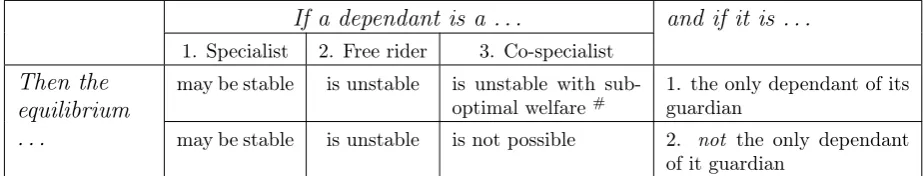
If the equilibrium is . . .
Then . . .
1. Any equilibrium 2. Stable 3. Unstable1. an agent which is the single dependant of its guardian is
either a specialist, free rider or co-specialist
a specialist either a specialist, free rider or co-specialist 2. agents that arenotsingle
de-pendants of their guardian are
all specialists or all free riders
[image:11.595.74.525.72.163.2]all specialists all specialists or all free riders
Table 2: This table describes efforts of dependant agents based on whether an equilibrium is stable or not.
Lemma 8 In a public goods game over a network G,
(a) The supporting agents in any equilibrium effort profile form a dominating set of the network.
(b) If a free rider leaves the network at equilibrium, then the equilibrium remains undisturbed.
(c) In any equilibrium, neighbours of a specialist free ride, whereby the specialists form an independent set of the network.
(d) In any equilibrium, neighbours of both co-specialists free ride, whereby co-specialist links form a matching of the network.
(e) Ifxis an equilibrium profile of efforts and di=|Ni|is the degree of the agent isuch that di >0,
then
xi≤e∗≤ Ei(x)≤die∗. (13)
Equality holds in the second inequality if agent iis not a free rider; further, equality holds in both the first and second inequality only if i is a specialist. The third inequality holds with equality if and only ifi is a free rider such that all its neighbours are specialists. Ifdi= 0, xi=Ei(x) =e∗.
Proof of Lemma 8: See Appendix
3.2
Networks with dependants
We now show a few results about the structure of the equilibria of public goods provision over a network containing at least one dependant-guardian pair. Recall that, in a network, if an agent i is adjacent to only one other agent j, then we call i a dependant of j (j is called the guardian of i). The link
(i, j)linking a dependant to its guardian is called a pendant line (a term borrowed from graph theory). If j and i are dependants of each other, we call them co-dependants. Table 2 the summarizes results regarding equilibria in networks which have at least one dependant-guardian pair. In Table 2, by stable equilibrium we mean stability under best-response dynamics (as defined and considered by [2]).
Proof of Table 2: Consider a game on a network having a guardian i with a dependant j. First consider an arbitrary equilibriumxof this game. Clearly, we have three possibilities: xj= 0(j is a free rider),xj =e∗ (j is a specialist) or0 < xj < e∗. Supposej is neither a specialist nor a free rider. By (EE(G)), Ej(x) =xj+xi=e∗, i.e.,iand j are co-specialists. Hence a dependant is either a specialist, free rider or co-specialist. We now show that if ihas in addition to j, another dependant, say k, then
j cannot be a co-specialist. Observe that k being a neighbour of co-specialist agentiis a free rider by Lemma 8(d). Hence Ek(x) = xi < e∗, which contradicts (EE(G)). Hence j can be either a specialist or a free rider but not a co-specialist. Since dj = 1, from (13), Ej(x) = e∗. If j is a free rider, then
Ej(x) =xi=e∗, i.e.,i is specialist, whereby all dependants ofiare free riders, by Lemma 8(c). And if
j is a specialist,iis a free rider (again by Lemma 8(c)), whereby from (EE(G)) every dependantk ofi
must exert efforte∗. Hence, dependants ofiare either all specialists (in which casei is a free rider) or
they are all free riders (in which caseiis a specialist).
If a dependant is a . . .
and if it is . . .
1. Specialist 2. Free rider 3. Co-specialist
Then the
equilibrium
. . .
may be stable is unstable is unstable with sub-optimal welfare #
1. the only dependant of its guardian
[image:12.595.70.532.72.160.2]may be stable is unstable is not possible 2. not the only dependant of it guardian
Table 3: This table describes the effect of the efforts of dependant agents on the stability of the equilibrium.
#A dependant can exist as a co-specialist in equilibrium only if it is the sole dependant of its guardian.
However this is not only an unstable equilibrium, but also yields suboptimal welfare. We show this in Theorem 13 later.
For unstable equilibria, the results follow from the discussion of arbitrary equilibria.
Observe that if a co-dependant pair exists, then only one of the two agents (who are both dependants) can be specialists whereby the equilibrium is always unstable. For better clarity, the results in Table 2 are reorganized in Table 3 putting in perspective the effect of the effort of a dependant at equilibrium on the stability of the equilibrium. Using the results in Tables 2 and 3, we have the result below regarding the non-existence of distributed equilibria in a network with at least one dependant.
Theorem 9 (Free riders in networks with dependants)
In a network with at least one dependant who is not a co-dependant, every Nash equilibrium always has a free-riding agent.
Proof : Suppose a guardian agentihas multiple dependants. Then by Table 2 (Row 2), either all the dependants ofi are free riders or they are all specialists; in the latter caseiitself is a free rider. Hence there exists at least one free rider.
Now suppose the guardian ihas only one dependantj such thatiandj are not co-dependants, i.e.,
i has another neighbour k. In this case, by Table 2 (Row 1), either (i) the j is a free rider (and i is a specialist) or (ii)j is a specialist (andi is a free rider), or (iii)iandj form a co-specialist pair. In the latter case, k is a free rider according to Lemma 8(d). Thus in every case, there always exists at least one free riding agent.
3.3
Forest networks
We now consider the structure of equilibria on forests. A network of agents is called a forest if there is no cycle between them. We refer the reader to [1] for a general introduction to forests and their properties. Here we recall that an induced subgraph of a forest is a forest and that a forest network can be represented as a disjoint union of trees (thus, for any two distinct trees in this union, there is no link in the forest having one vertex in each tree).
A vertex in a graph is isolated if it has degree zero (i.e., no neighbours). A link is said to be isolated if both vertices in the link have degree unity. Note also that a tree which is not an isolated vertex has at least two dependants [1]. The following lemma is the interpretation of our previous graph theoretic results Lemma 6(c) and Lemma 9 from [7], in that order, in the context of public goods provision over networks.
Lemma 10 (Structure of equilibria in forest networks)
For a public goods game over a forest networkG,
(a) If the game admits a distributed equilibrium, then the network is a disjoint union of isolated links and isolated agents.
(b) The supporting agents in any equilibrium are either specialists or co-specialists.
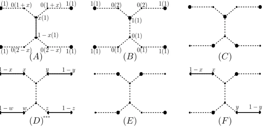
Figure 2: This figure shows six different equilibria of a public goods game over a tree network of 10 agents. A dotted line between agents indicates adjacency. Agents denoted by large black circles are specialists, whereas those denoted by small black circles are free riders. A solid line between adjacent agents indicates a co-specialist link, with black semicircles denoting the co-specialist agents. (B), (C)
and(E)are specialized equilibria, whereas(A), (D)and(F)are hybrid equilibria. For an agentiof the network, the number denotes the normalized effort e1∗xiexerted by it at equilibrium while the normalized
effort of the closed neighbourhood Ei(e1∗x) is mentioned for equilibria (A) and (B) are mentioned in
parenthesis. Observe that e1∗xi ≥0, Ei( 1
e∗x) ≥ 1 and at least one of the two inequalities is tight, as
indicated by (EE(G)).
∗∗∗ In equilibrium(D), x+y≥1 andw+z≥1are necessary for it to be an equilibrium.
(d) The cost of the equilibrium effort profile is
ce∗ #(specialists) +12#(co−specialists)
,
where #(·)is stands for “number of ”.
Proof :
(a) Consider a forest network G which is a disjoint union of m trees T1, . . . , Tm, such that G
ad-mits a distributed equilibriumx. Then, since the trees T1, . . . , Tm are disjoint, the subvectorxTk
corresponding to efforts of agents in Tk is a distributed equilibrium overTk for allk.
For some k, let agent j be a dependant in Tk and let i be the guardian of j. If Tk has more than two agents, we must have di >1 (since Tk is a connected graph), whereby i and j are not co-dependants. Hence Tk satisfies the condition in Lemma 9. This contradicts the possibility of a distributed equilibrium xTk. Hence for any k, Tk must consist of at most two agents. HenceG
consists of isolated links and isolated agents.
(b) Let x∈NE(G). The network of supporting agentsGsupp(x) is also a forest since it is an induced
subgraph of the forestG. Letxsupp(x)denote the efforts exerted by the supporting agents. Observe
that from Lemma 8(b), it follows that xsupp(x) is an equilibrium for the public goods game over
the forest Gsupp(x). Moreover, this equilibrium is distributed. Now, from Lemma 10(a), it follows
that Gsupp(x) consists only of isolated links and isolated vertices. The isolated links correspond to
co-specialist links whereas the isolated vertices correspond to specialists. This proves the claim.
(c) By Theorem 7, we know that 1
e∗xsolvesLCP(G). We know from Lemma 5(b) that if the network
is a forest, there always exists a maximal independent set S ⊆supp(1
e∗x) = supp(x). The agents
inS form a specialized equilibrium given byy:=e∗
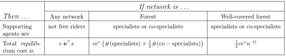
If network is . . .
Then . . .
Any network Forest Well-covered forestSupporting agents are
not free riders specialists or co-specialists specialists or co-specialists
Total equilib-rium cost is
ce⊤x ce∗ #(specialists) + 1
2#(co−specialists)
1
[image:14.595.74.548.70.163.2]2ce∗n††
Table 4: Summary of roperties of supporting agents as described in Lemma 10.
†† Follows from Theorem 3(b), proved later in Section 6.
From Lemma 10(b) above, we know that the supporting agents in x are either specialists or co-specialists. Let agent k be a specialist in the equilibrium x. We first show that k is also a specialist in y. Observe that if k is not a specialist in y, then k is a free rider. Hence
Ek(y) = Pk′∈supp(y)akk′yk′ ≤ Pk′∈supp(x)akk′yk′ = 0, since by Lemma 8(c), k has no
neigh-bours in supp(x). This means that y does not satisfy (EE(G)); a contradiction to y being an equilibrium. Every specialist inxis a specialist iny.
Now let i and j be co-specialists inx. We now show that exactly one of i and j specializes in y
whereas the other free rides. By Lemma 8(c), it is clear that both i and j cannot be specialists in y, since they are adjacent in G. On the other hand, suppose both iand j are free riders in y. Then,Ei(y) =Pk′∈supp(y)aik′yk′ ≤Pk′∈supp(x)aik′yk′ =yj+Pk′∈supp(x)\{j}aik′yk′ = 0,since by
Lemma 8(d) neighbours of co-specialists free ride, whereby i has no neighbours in supp(x) other thanj.
Thus, out of every pair of co-specialists inx, one agent specializes in the specialized equilibriumy, while the other free rides. This substitution of effort between co-specialists requires the same total effort. Hence, the equilibrium cost
ce⊤x=c #(specialists inx) +12#(co−specialists inx)
=c# (specialists iny) =ce⊤y, (14)
i.e., the cost incurred by both equilibria is the same.
(d) This was shown in (14) above.
Lemma 10(b) means that in an equilibrium xin a public goods game over a forest, if an agent i is neither a specialist nor a free rider, i.e.,0< xi < e∗, then there always exists a neighbourj ofithat is a co-specialist ofiin equilibriumxand, in another equilibrium, substitutes the deficit of the effort of i. In the specialized equilibrium described in part (c), in every co-specialist pair, one agent specializes to substitutes the effort of its co-specialist, who then free rides. The results in Lemma 10 are summarized in Table 4.
In Figure 2, various equilibria on a tree network are shown. Notice that (B)and(E)are specialized equilibria contained in the support of equilibria(A)and(D)respectively.
4
Refinement of the equilibrium based on weighted total effort
and cost
In this section, we prove Theorem 2 and compare equilibria based on their total weighted effort and the total cost incurred, and study how the structure of the network affects the existence of an optimum specialized equilibrium. The cost incurred by an equilibrium isce⊤x, whereas for a set of weightswi ≥0, the w-weighted effort isw⊤x. Recall from the discussion in the introduction that although the above
functions for ranking equilibria are linear, finding the optimum equilibrium is a hard problem.
Proof of Theorem 2
(a) Let S∗ be the maximum w-weighted independent set in G. We need to show that e∗1
S∗ is a
equilibrium profile. By Theorem 7 we know that e1∗xsolves LCP(G), whereby from Theorem 4(b)
we can say that
E∗
w= max
w⊤xx∈NE(G) = max
w⊤e∗y ysolves LCP(G) =e∗αw(G).
Since wi ≥ 0 for all i ∈ V, S∗ is also a maximal independent set. As a consequence e∗1S∗ is a
specialized equilibrium, and its weighted effort is e∗w⊤
1S∗ = e∗αw(G), by definition of the w -weighted maximum independent set. It follows that e∗
1S∗ attains the maximum total weighted
equilibrium effort and hence E∗w=ES∗
w.
(b) Observe that the minimum cost in equilibrium is given by,
C∗=c·mine⊤xx∈NE(G) =c·e∗min
e⊤x
xsolves LCP(G) .
By Theorem 4(d) we can say that if the network Gis a forest, the above quantity isce∗β(G). Let
S′ denote the smallest maximal independent set ofG, thene∗1
S′ is a specialized equilibrium which
incurs a cost ce∗e⊤1
S =ce∗β(G). Hence if the network is a forest, we have thatC∗ =CS∗, and
e∗1
S′ incurs the minimum cost.
(c) We first show a more general result: If y is an equilibrium and a subset S ⊆ supp(y) of the supporting agents ofy form a maximal independent set of the network, then the specialized equi-librium supported onS requires total effort at least as much as that ofy, i.e.,e∗|S| ≥P
jyj. Let
U := supp(y)\S. Then, from (EE(G)),∀i∈supp(y),
Ei(y) = X j∈V
aijyj+yi=e∗.
Summing over i∈S gives,
X i∈S
X j∈V
aijyj+e⊤y− X j∈U
yj =e∗|S|.
Thus,
e∗|S| −e⊤y(=a)X
i∈S X j∈U
aijyj− X j∈U
yj = X j∈U
(|NS(j)| −1)yj
(b)
≥0.
The equality in (a)follows from the observation thataij is nonzero fori∈S only ifj /∈S due to
S being an independent set. Moreover, in this setV\S,yj is non-zero only forj∈U. Now, since
S is a maximal independent set, every vertex not in S has at least one neighbour in S whereby
|NS(j)| ≥1and justifies the inequality(b).
Now, if the network is such that it admits a distributed equilibrium, all the agents in the network are supporting agents of this equilibrium whereby the support of any specialized equilibrium is clearly its subset. Following the discussion above, we can say that the cost of a distributed equilibrium is at most as much as that of any specialized equilibrium, i.e.,CD∗≤CS∗.
(d) By Lemma 5(a), we know that if the network is regular, e
d+1 is a solution toLCP(G) such that
it minimizes the function e⊤xamongst all solutions of LCP(G). It follows from Theorem 7 that
e∗ e
d+1 is a distributed equilibrium of the public goods game of the regular network with minimum
cost, wherebyC∗=CD∗. This proves the Theorem 2(d).
5
Refinement of the equilibrium based on welfare
In this section we prove Theorem 1 by studying the welfare of specialized equilibria. We establish conditions on the concavity of the benefit function and on the structure of the underlying network for which there exists a specialized equilibrium which yields maximum equilibrium welfare. Moreover, we also give the specialized equilibrium which yields optimal welfare, under these conditions.
the Nash equilibrium of the public goods game over a network, when searching for welfare maximizing equilibria.
While proving Theorem 1 we first show bounds on the welfare of equilibrium profiles thereby estab-lishing a range for the maximum equilibrium welfare. We then show the convergence of these bounding functions to identify the behaviour of the welfare function and the maximum equilibrium welfare as the concavity of the benefit function varies. While varying the concavity of the benefit function, we keep
b(e∗)andb′(e∗)fixed whereby the equilibra remain unchanged.
To this end, for µ∈Rn, define,
θµ:= max{µ⊤x|x∈NE(G)} and θµS:= max{µ⊤x|x∈SNE(G)}.
Lemma 11 Forµ∈Rn,θµ andθSµ are continuous functions ofµ.
Proof : Observe that θµ and θSµ are both value functions of the optimization of a continuous function
µ⊤xover setsNE(G)andSNE(G)that are compact as well as independent ofµ. If follows from stability
results in optimization theory, such as [4, Thm. 7], that bothθµ and θSµ are continuous.
For the rest of the section, we assume that the network does not have any isolated agents, i.e.,di≥1 for allias assumed in the statement of the theorem. Define
σj :=
b(dje∗)−b(e∗)
ce∗(dj−1) ifdj>1, σb ifdj= 1.
and σj′ :=
1
cb′(dje∗) ifdj >1,
σb ifdj = 1.
Ifdj >1, observe thatσjdenotes the normalized4slope of the secant between(e∗, b(e∗))and(dje∗, b(dje∗)), whileσ′
j denotes the normalized slope of the tangent to the benefit functionb at the pointdje∗. These have been depicted in Figure 3 for clarity. Let lj = (σj+Piaijσi−1) and uj = (σ′j+
P
iaijσi′−1). Denote byσ, σ′, land uthe corresponding vectors withncomponents.
In establishing Theorem 1, we need to be able to formally relate W∗Uto changes in σb. We also note
that while the limiting behaviour ofWUasσb→1 is known from [2, Prop 1], it does not automatically yield a proof of Theorem 1. The following theorem provides linear upper and lower bounds on the welfare of equilibrium effort profiles and the maximum equilibrium welfare. These bounds are essential in the proof of Theorem 1.
Theorem 12 For a public goods game over a network without isolated agents, if x is an equilibrium effort profile,
(a) The welfare function is bounded as follows,
cl⊤x≤WU(x)−nb(e∗) +ce∗e⊤σ≤c u⊤x+ce∗d⊤ σ−σ′, (15)
whereby,
cθl≤W∗U−nb(e∗) +ce∗e⊤σ≤cθu+ce∗d⊤ σ−σ′, (16)
and similarly ,
ce∗θlS≤W
S∗
U −nb(e∗) +ce∗e⊤σ≤ce∗θ S
u+ce∗d⊤ σ−σ′
. (17)
(b) Keepingb′(e∗)andb(e∗)fixed and varying σ
b, we have that,
lim
σb→1
lj = lim σb→1
uj=dj, for allj, (18)
lim
σb→0
lj= lim σb→0
uj =−1, for all j, (19)
lim
σb→0
σj−σ′j= lim σb→1
σj−σj′ = 0, for allj. (20)
(c) Keepingb′(e∗)andb(e∗)fixed and varying σ
b, we have that,
lim
σb→1
WU(x) =n b(e∗)−ce∗+cd⊤x,
lim
σb→0
WU(x) =nb(e∗)−ce⊤x.
4Normalization refers to division by
Proof :
(a) From Lemma from 8(e), we know that for an equilibrium profile of effortsx,e∗≤ E
i(x)≤dje∗ for agentsj withdj >1. Due to the concavity of the benefit function, the tangent atdje∗always lies above the function whereas the secant between(e∗, b(e∗))and(d
je∗, b(dje∗))always lies below the function for the interval[e∗, d
je∗](see Figure 3). Hence we have,
b(e∗) +cσj(Ej(x)−e∗) ≤ b(Ej(x)) ≤ b(dje∗)−cσ′j(dje∗− Ej(x)), (21)
⇐⇒ cσjEj(x) ≤ b(Ej(x))−b(e∗) +cσje∗ ≤ cσj′Ej(x) +ce∗dj(σj−σj′), (22)
where the equivalence follows from the equation b(dje∗) =b(e∗) +cσje∗(dj−1) and subtracting
b(e∗)−cσ
je∗ from all sides. For the case where dj = 1, it can be seen from Lemma 8(e), that
Ej(x) = e∗ whereby b(Ej(x)) = b(e∗), i.e., (21) holds for agents who are dependants. Now since
WU(x) =Pj∈V b(Ej(x))−cxj, the sum of the inequalities in (22) for all agentsj, gives
cX
j
(σjEj(x)−xj)≤WU(x)−nb(e∗) +ce∗e⊤σ≤c
X j
(σj′Ej(x)−xj) +ce∗dj(σj−σj′).
Observe that,
X j
σjEj(x)−xj:= X
j
σj(xj+ X
i
aijxi)−xj= X
j
(σj−1)xj+ X
j
σj X
i
aijxi
(c)
=X
j
(σj−1)xj+ X
i
xi X
j
aijσj
(d)
=X
j
σj−1 + X
i
aijσi
xj =l⊤x,
where the equality in(c)is due to interchanging the order of summation and the equality in(d)holds by exchange of summation indicesiandj. Following a similar argument,we getP
jσ′jEj(x)−xj=
u⊤x. The bounds on W
U(x)−nb(e∗) +ce∗e⊤σ follow directly. Moreover, the bounds on the
maximum equilibrium welfare W∗U in (16) and the maximum specialized equilibrium welfare WSU∗
in (17) follow after maximizing all quantities in (15) over NE(G)andSNE(G), respectively.
(b) We first show the intermediate limits,
lim
σb→1
σj = lim σb→1
σ′
j= 1, and lim σb→0
σj = lim σb→0
σ′
j= 0, for allj.
Since lj, uj and σj−σj′ are linear functions of σ and σ′, by the sum law of limits, showing the above limits is sufficient to prove the limits in the statement of the theorem.
Case I: (dj = 1) Clearly, by definition σj =σ′j =σb, whereby the limits hold trivially for both
σb→0 andσb→1.
Case II: (dj >1) First consider the caseσb →1. To show the limit ofσj, observe that σj ≥σb sincebis increasing and concave. Moreover, by the concavity ofb, the tangent ate∗ lies above the
function, i.e.,
b′(e∗)(d
j−1)e∗+b(e∗)≥b(dje∗). (23) Sinceb′(e∗) =c, rearranging, we haveσ
j≤1. Now sinceσj≥σb,we getlimσb→1σj = 1.
For computinglimσb→1σ
′
j, letσ∗denote the normalized slope of the secant between(e∗, b(e∗))and
(n−1)e∗, b((n−1)e∗)
. Observe that sincebis increasing and concave, we again have1≥σ∗≥σb,
whereby we have limσb→1σ
∗= 1.
Since1≤dj≤n−1for any j, by the concavity ofb, we have,
b′(e∗)≥b′(d
je∗)≥b′ (n−1)e∗. (24) Moreover, an inequality similar to (23) with the tangent to bat(n−1)e∗ gives,
b′((n−1)e∗)≥ 1
e∗(b(ne
∗)−b((n−1)e∗)) = 1
e∗(b(e
∗) +e∗c(n−1)σ
b−(b(e∗) +e∗c(n−2)σ∗)),
whereby σj′ ≤1. Hence combining with (24) gives,limσb→1b
′(d
je∗)≥climσb→1 (n−1)σb−(n−
2)σ∗)
=c, whereby,limσb→1σ
′
j ≥1. Sinceσj′ ≤1,limσb→1σ
′
Figure 3: Bounds on b(Ei(x))for j such thatdj >1 as given by the inequality in (21). The tangent and secant have slopescσ′
j andcσj respectively. Due to concavity of the functionb, the tangent always lies above the function and the secant always lies below the function for the interval [e∗, d
je∗]. Hence
b(e∗) +cσ
j Ej(x)−e∗
andb(dje∗)−cσ′j dje∗− Ej(x)
are the bounds. In the case wheredj= 1, both quantities becomeb(e∗)
To show the limits of σj andσj′ as σb→0, fordj>1, we need the following set of inequalities,
0≤σ′
j ≤σj≤σb
n−1
dj−1
. (25)
Observe that the first and second inequality follow from the monotocity and concavity ofb. The third inequality follows from 0 ≤b(ne∗)−b(d
je∗) =b(ne∗)−b(e∗)− b(dje∗)−b(e∗)=σb(n−
1)e∗−σ
j(dj−1)e∗. Hencelimσb→0σj= limσb→0σ
′
j= 0. (c) Applying limits to the result in part (a), we have that
lim
σb→1
cl⊤x≤ lim
σb→1
WU(x)−nb(e∗) +ce∗ lim
σb→1
X j
σj≤ lim σb→1
cu⊤x+ lim
σb→1
ce∗d⊤(σ−σ′),
and
lim
σb→0
cl⊤x≤ lim
σb→0
WU(x)−nb(e∗) +ce∗ lim
σb→0
X j
σj≤ lim σb→0
cu⊤x+ lim
σb→0
ce∗d⊤(σ−σ′).
Applying the limits from part (b) proves the result.
Proof of Theorem 1
(a) Let x∗ be the specialized equilibrium as mentioned in the statement of the theorem, whereby
x∗=e∗
1S, using Theorem 7. The limiting value of the welfare at this equilibrium, using Theorem 12(c) is,
lim
σb→1
WU(x∗) =n(b(e∗)−ce∗) +ce∗
X j∈S
dj=n(b(e∗)−ce∗) +ce∗αd(G), (26)
sinceS is ad-weighted maximum independent set in the network. We now calculate the limiting value ofW∗Uusing (16), i.e.,
lim
σb→1
cθl≤ lim σb→1
WU∗−nb(e∗) +ce∗e⊤σ≤ lim
However, as a consequence of Theorem 12(b), limσb→1l = limσb→1u=d, whereby using Lemma
11,limσb→1θl= limσb→1θu=θd. Moreover, sinced≥0,θd=e
∗α
d(G)by Theorem 4(b). Hence
lim
σb→1
W∗U=n b(e∗)−ce∗
+ce∗αd(G). (27)
Hence limσb→1W
∗
U= limσb→1WU(x
∗).Now, sinceW∗
U≥W S∗
U ≥WU(x∗), taking limits on all three
quantities gives
lim
σb→1
W∗U≥ lim
σb→1
WUS∗≥ lim
σb→1
WU(x∗)
Since the limiting values ofW∗
U andWU(x∗)are the same, the above inequality proves the result.
(b) Consider a forest G and let x′ be the specialized equilibrium as mentioned in the statement of
the theorem, whereby x′ = e∗1
S′, using Theorem 7. The limiting value of the welfare at this
equilibrium, using Theorem 12(c) is,
lim
σb→0
WU(x′) =nb(e∗)−ce∗
X j∈S′
1 =nb(e∗)−ce∗β(G), (28)
since S′ is the smallest maximal independent set in the network, i.e., cardinality of S′ is β(G).
Now, to calculate the limiting value ofW∗U, applying limits to (16) gives,
lim
σb→0
cθl≤ lim σb→0
WU∗−nb(e∗) +ce∗e⊤σ≤ lim
σb→0 cθu.
However, from Theorem 12(b) limσb→0l = limσb→0u= −e, whereby using Lemma 11, we have
limσb→0θl= limσb→0θu=θ−e. Now observe that,
−θ−e= min{e
⊤x|x∈NE(G)}=e∗min{e⊤y|y solves LCP(G)}.
Moreover, since G is a forest, we know from Theorem 4(d), that min{e⊤x|xsolves LCP(G)}=
β(G). Hence
lim
σb→0
W∗U=nb(e∗)−ce∗β(G), (29)
whereby limσb→0W
∗
U = limσb→0WU(x
′). Since W
U ≥ WSU∗ ≥ WU(x′), taking limits on all three
quantities and arguing as in part (a) gives the result. (c) Let the networkGadmit a distributed equilibriumx∗, i.e.,x∗
i >0for alli. It follows from (EE(G)) that for anyx∗,E
i(x) =e∗ for all agentsi. HenceWU(x∗) =nb(e∗)−ce⊤x∗, which is independent
of variation inσb (recall that keepingb(e∗)andb′(e∗)fixed asσb varies ensures that the equilibria are unaltered).
LetSbe a maximal independent set ofG, wherebye∗
1S is a specialized equilibrium. From Theorem 2(c), the costce⊤x∗ incurred by the distributed equilirium is at most as much as the costce∗|S|
incurred by the specialized equilibrium e∗1
S, i.e.,ce∗|S| ≥ce⊤x∗ or equivalently,
WU(x∗)≥nb(e∗)−ce∗|S|.
Observe that this holds true for any x∗ ∈DNE(G) and any maximal independent set S, i.e., the
variable S in the RHS is independent of the variablex∗ in the LHS. Hence, we may infimize over
x∗ and maximize overS, leading to,
inf{WU(x∗)|x∗∈DNE(G)} ≥max{nb(e∗)−ce∗|S| |e∗1S ∈SNE(G)},
WDU∗≥nb(e∗)−ce∗min{|S| |S is maximal independent},
=nb(e∗)−ce∗β(G). (30)
The limiting value ofWS∗
U using (17) is,
lim
σb→0 cθS
l ≤ lim σb→0
WSU∗−nb(e∗) +ce∗e⊤σ≤ lim
σb→0 cθS
u.
Now, as in part (b),limσb→0l= limσb→0u=−e, wherebylimσb→0W S∗
U =nb(e∗)+cθ S
−e. Moreover,
again as in part (b),
−θS−e= min{e
⊤x|x∈SNE(G)}=e∗min{|S| |S is maximal independent}=e∗β(G),
sinceβ(G)is the cardinality of the smallest maximal independent set ofG. Hence,
lim
σb→0
WSU∗=nb(e∗)−ce∗β(G). (31)
Figure 4: Examples of well-covered networks. The vertices marked by larger circles form maximal independent sets. All maximal independent sets in the well-covered tree network consist of 4 agents while those in the cycle network consist of 3 agents respectively. Observe that the well-covered tree over 8 agents depicted in the figure has exactly 4 guardian-dependant pairs such that exactly one of the two is part of any maximal independent set.
6
Welfare and cost in well-covered forest networks
In this section we prove Theorem 3. A networkGis said to be well-covered if all its maximal independent sets have the same cardinality, i.e., α(G) = β(G). Figure 4 shows example networks which are well-covered.
Before proceeding to the proof, we show a more general result regarding the role of dependants on the efficiency of the equilibrium. This result is put to use while proving Theorem 3(a).
Theorem 13 (Co-specialist pendant lines are inefficient)
In a public goods game, if a guardian has a single dependant, then in an equilibrium yielding maximum equilibrium welfare, exactly one of the guardian-dependant pair specializes whereby the other free rides.
Proof : Recall from Table 2 (Row 1, Column 1), that if a guardian has a single dependant, then either one of the guardian or dependant free rides or they both form a co-specialist pair. Note that an equilibrium where the guardian-dependant pair form a co-specialist link is not possible if the guardian has multiple dependants (See Table 3 (Row 2, Column 3)). We have to show that if the guardian-dependant pair form a co-specialist link, then the equilibrium yields suboptimal welfare. We affirm this by showing the existence of another equilibrium which yields higher welfare.
Let agent i be the only dependant of agent j such that they are not co-dependants. Let x be an equilibrium such thatiandjform a co-specialist link, i.e.,xi+xj =e∗. From Lemma 8(d), we can infer that all the neighbours ofj other thani free ride in the equilibriumx, i.e.,
xk = 0, ∀ k∈Nj\{i}. (32)
Now, consider the profile of efforts y, where yj =e∗, yi = 0 and for all other agents kexert the same effortyk=xk. We first showy∈NE(G)and then prove that indeedWU(y)> WU(x).
Observe that for all agents k other than j and its neighbours, the effort of closed neighbourhood remains unchanged, i.e.,yk=xk, andEk(y) =Ek(x),whereby,
yk≥0, Ek(y)≥e∗, yk(Ek(y)−e∗) = 0, ∀ k /∈ {j} ∪Nj, (33)
from (EE(G)) sincexis an equilibrium. Now, for agentj,
yj=e∗, andEj(y) =yj+yi+ X k∈Nj\{i}
yk=e∗+ 0 + X k∈Nj\{i}
xk =e∗,
by (32). Moreover we have that,
yk=xk= 0, andEk(y) =yj+ X r∈Nk\{j}
yr≥e∗, ∀k∈Nj\{i},
sinceyr≥0 for allr, and
![Figure 1:This figure (not to scale) describes the two extreme cases of concavity. Observe that asσb → 1, the benefit function is nearly linear in the interval [e∗, ne∗] and having slope b′(e∗), whereas asσb → 0, the benefit function plateaus](https://thumb-us.123doks.com/thumbv2/123dok_us/252677.524699/5.595.163.433.68.188/describes-concavity-observe-function-interval-benet-function-plateaus.webp)