Munich Personal RePEc Archive
Quasi Maximum Likelihood Analysis of
High Dimensional Constrained Factor
Models
Li, Kunpeng and Li, Qi and Lu, Lina
20 December 2016
Online at
https://mpra.ub.uni-muenchen.de/75676/
Quasi Maximum Likelihood Analysis of High Dimensional
Constrained Factor Models
∗Kunpeng Li†, Qi Li‡ and Lina Lu§
September 25, 2016
Abstract
Factor models have been widely used in practice. However, an undesirable feature of a high dimensional factor model is that the model has too many parameters. An effective way to address this issue, proposed in a seminar work by Tsai and Tsay (2010), is to decompose the loadings matrix by a high-dimensional known matrix multiplying with a low-dimensional unknown matrix, which Tsai and Tsay (2010) name the con-strained factor models. This paper investigates the estimation and inferential theory of constrained factor models under large-N and large-T setup, where N denotes the number of cross sectional units andT the time periods. We propose using the quasi maximum likelihood method to estimate the model and investigate the asymptotic properties of the quasi maximum likelihood estimators, including consistency, rates of convergence and limiting distributions. A new statistic is proposed for testing the null hypothesis of constrained factor models against the alternative of standard factor mod-els. Partially constrained factor models are also investigated. Monte carlo simulations confirm our theoretical results and show that the quasi maximum likelihood estimators and the proposed new statistic perform well in finite samples. We also consider the extension to an approximate constrained factor model where the idiosyncratic errors are allowed to be weakly dependent processes.
Key Words: Constrained factor models, Maximum likelihood estimation, High dimensionality, Inferential theory.
JEL #: C13, C38.
∗We would like to thank the guest editors and two anonymous referees for their insightful comments
that greatly improve our paper. We also thank Jushan Bai for the helpful comments on an early version of this paper. Kunpeng Li gratefully acknowledges the financial support from China NSF No.71571122 and No.71201031. Qi Li’s research is partially supported by China NSF project No.71133001 and No 71601130.
†International School of Economics and Management, Capital University of Economics and Business,
Fengtai District, Beijing, 100070, China. Email: [email protected].
‡Corresponding author: Qi Li, Email: [email protected]. Department of Economics, Texas A&M
Uni-versity, College Station, TX 77843, USA; International School of Economics and Management, Capital University of Economics and Business, Beijing, China.
1
Introduction
With the rapid development of data collection, storing and processing techniques in com-puter science, econometricians and statisticians now face large dimensional data setups more often than ever before. A challenge along with the appearances of large data is how to extract useful information from data, or put differently, how to effectively conduct di-mension reduction on data. Factor models are proved to be an effective way to perform this task. Over the last three decades, the literature has witnessed wide applications of factor models in many economics disciplines. In finance, Conner and Korajczyk (1986, 1988) and Fan, Liao and Shi (2014) use factor models to measure the risk and performance of large portfolios. In macroeconomics, Geweke (1977) and Sargent and Sims (1977) use dynamic factor models to identify the source of primitive shocks. In labor economics, Heckman, Stixrud and Urzua (2006) use factor models to capture unobservable personal abilities. In international economics, Kose, Otrok and Whiteman (2003) use multilevel factor models to separate global business circles, regional business circles and country-specific business circles. Large dimensional factor models are also used in a variety of ways to deal with strong correlations, see e.g., Fan, Liao and Mincheva (2011) and Fan, Liao and Mincheva (2013), among others.
A standard factor model can be written as
zt=Lft+et, t= 1,2, . . . , T,
wherezt= (z1t, . . . , zN t)′ is a vector ofN variables at timet,Lis anN×rloadings matrix,
ft is anr-dimensional vector of factors andet is anN-dimensional vector of idiosyncratic
errors. The traditional (classical) factor analysis assumes that N is fixed and T is large. This assumption runs counter to usual shape of large dimensional data sets, in whichN is usually comparable to or even greater thanT (Stock and Watson (2002)). Recent literature contributes a lot to the asymptotic theory with N comparable to or even greater than T. Bai and Ng (2002) propose several information criterions to determine the number of factors in a large-N and large-T environment. Under a similar setup to Bai and Ng (2002), Stock and Watson (2002) prove that the principal components (PC) estimates are consistent in approximate factor models of Chamberlain and Rothschild (1983). Bai (2003) moves forwards along the work of Stock and Watson (2002) and gives the asymptotic representations of the PC estimates of loadings, factors and common components. Doz, Giannone and Reichlin (2012) consider the maximum likelihood (ML) method and prove the average consistency of the maximum likelihood estimates (MLE). Bai and Li (2012, 2016) use five different identification strategies to eliminate the rotational indeterminacy from asymptotics and give limiting distributions of the MLE. Fan, Liao and Wang (2014) propose a new projected principal component method to more accurately estimate the unobserved latent factors.
estimated within the model, which makes it difficult to analyze and interpret the economic implications of the estimates. However, if the space of the loading matrix is spanned by a low dimension matrix, this problem can be much ameliorated. In this paper, following Tsai and Tsay (2010), we address this problem by considering the following constrained factor model
zt=MΛft+et,
whereM is aknownN ×k matrix with rankkand Λis ak×r unknown loadings matrix with rankr. We assumer < k≤C for some generic constantC. In the above specification, M consists of the bases of the loading matrix. The underlying true loadings are a weighted average of these bases associated with the weights matrixΛ, which are the parameters of interests. The number of loading parameters now iskr instead of N r. So the number of parameters is greatly reduced.
Our work is closely related to Tsai and Tsay (2010) who were the first to consider con-strained factor models. This paper differs from Tsai and Tsay (2010) in several dimensions. First, although Tsai and Tsay propose using PC and ML methods to estimate constrained factor models, their asymptotic analysis focuses only on the PC method. They obtain convergence rates of the PC estimates. As a comparison, we investigate asymptotics of the ML method and derive the convergence rates and limiting distributions of the MLE. Given the limiting distributions, one can easily construct (1−α)-confidence intervals if prediction is the target of interest, or use t-test or F-test to conduct statistical inferences on the underlying parameter values if hypothesis testing is the purpose. Second, Tsai and Tsay consider the setup thatkis large (but still smaller thanN). In this paper, we instead assume that k is fixed①
. In our viewpoints, assuming a fixed k is of practical and theo-retical interests. In some typical examples, the parameter kis interpreted as the number of groups or categories, according to which the variables are classified (see Tsai and Tsay (2010)). This value is usually not large in real data. Therefore, a fixed-k assumption is adopted in this paper. Furthermore, in constrained factor models, a largekleads to a larger number of parameters being estimated. The estimation accuracy is reversely linked withk for a given sample size. Whenk is large, the benefit of constrained factor models against standard factor models becomes weak, which makes constrained factor less attractive in practice. Third, an importantly related issue in constrained factor models is on conducting valid model specification check on the presence of matrix M. Tsai and Tsay consider the traditional likelihood ratio test to perform this task. But the traditional likelihood ratio test is designed under fixed-N and large-T setup, which conflicts to large-N and large-T scenarios. In this paper, we propose new statistics for testing model specifications that are applicable to the large-N and large-T setups.
The rest of the paper is organized as follows. Section 2 provides more empirical examples
①
of the constrained factor model. Section 3 introduces the model and lists the assumptions needed for the subsequent analysis. Section 4 delivers the consistency and limiting distribu-tion results of the MLE. Secdistribu-tion 5 considers testing issues within constrained factor models. Section 6 considers a partially constrained factor model and presents the asymptotic prop-erties of the MLE for this model. Section 7 presents the Expectation-Maximization (EM) algorithm to implement the QML estimation. Section 8 conducts Monte Carlo simulations to investigate the finite sample performance of the MLE and to study the empirical size and power of the proposed model specification test. In Section 9, we relax Assumption B to allow for the idiosyncratic errors to have a more general weakly dependence structure. Section 10 concludes the paper. All technical contents are delegated to several appendices.
2
Motivating Applications
The well-known equilibrium arbitrary pricing theory (APT) implies that the observed assets returns can be expressed into a linear factor structure, see Ross (1976), Conner and Korajczyk (1988) among others. This motivates the use of the following factor model
rit = r
∑
j=1
lijfjt+eit
to study the performance of portfolios, whererit is the excess return of the ith security at
time t, fjt denotes the jth risk premium at time t and lij the beta coefficient of the jth
risk premium for security i. However, as pointed out by Rosenberg (1974), the common movements among the assets returns may be related with the individual characteristics. Such characteristics include capitalization and book-to-price ratios as suggested in Fama and French (1993), momentum as in Carhart (1997), own-volatility as in Goyal and Santa-Clara (2003). Letxipdenote the observedpth characteristic of theith security. Rosenberg
(1974) considers the specification
lij = k
∑
p=1
xipλpj+vij, or L=MΛ +V,
where M = (xip)N×k is the observed characteristics matrix. Rosenberg’s specification is
very close to the one studied in this paper. With a slight modification, the analysis in this paper can easily be extended to cover the Rosenberg’s model.
A limitation of Rosenberg’s specification is that the factor betas are assumed to be linear functions of the observed characteristics, which is overly restrictive in practice. To accommodate this concern, Conner and Linton (2007) and Conner, Hagmann and Linton (2012) consider the following nonparametric specification
lij =gj(xij).
where gj(·) is an unknown smooth function. Conner, Hagmann and Linton (2012) apply
of the characteristics. However, an undesirable feature in these two papers is that the estimation of the model involves an iterative procedure between the factors and unknown functions, which is formidable to many applied researches. To address this issue, we in-stead consider using a series of polynomial functions to approximate the unknown function gj(·). More specifically, we consider approximating the functiongj(·)by all the polynomial
functions with power less thanq, i.e.,
gj(x)≈λj0+λj1x+· · ·+λjqxq. (2.1)
Given this, the model now can be written asL=MΛ with
M =
1 x11 x211 · · · xq11 · · · x1r x21r · · · xq1r
1 x21 x221 · · · xq21 · · · x2r x22r · · · xq2r
..
. ... ... . .. ... . .. ... ... ... . .. ...
1 xN1 x2N1 · · · xNq1 · · · xN r x2N r · · · xqN r
and
Λ =
λ10 λ11 · · · λ1q 0 · · · 0 · · · 0 · · · 0
λ20 0 · · · 0 λ21 · · · λ2q · · · 0 · · · 0
..
. ... . .. ... ... . .. ... . .. ... ... . .. ... λr0 0 · · · 0 0 · · · 0 · · · λr1 · · · λrq
′
.
The above model can be viewed as a special case of the constrained factor model with some zero restrictions imposed on Λ. The model considered here maintains the nonlinear function feature of Conner and Linton (2007) and Conner, Hagmann and Linton (2012) but the computational burden has been much reduced. A primary issue related with our method is whether the approximation (2.1) is good enough. This work can be partially addressed by theW statistic proposed in Section 5.
3
Constrained Factor Models
Let N denote the number of variables and T the sample size in the time dimension. We consider the following constrained factor model
zt=MΛft+et, (3.1)
wherezt= (z1t, z2t, . . . , zN t)′ is an N-dimensional vector of explanatory variables at time
t;M is a specifiedN×k(known) matrix with rankk;Λis the k×rloading matrix of rank r; ft = (f1t, f2t, . . . , frt)′ is a vector of r latent common factors; et is an N-dimensional
vector of idiosyncratic disturbances and is independent of ft. Throughout the paper, we
assume k≥r. If k < r, we can simply consider the linear regression zt= M ft∗+et with
f∗
t = Λft. The model effectively becomes a factor model with k (whenk < r) factors.
Our analysis is based on similar assumptions used in standard factor models, see Bai and Li (2012) for the asymptotic analysis of the MLE for standard high dimensional factor models. The symbolCappearing in the following assumptions denotes a generic constant. Our assumptions include:
Assumption A: {ft} is a sequence of fixed constants with f¯ = ∑Tt=1ft = 0. Let
Mff = T1 ∑Tt=1ftft′ be the sample variance of ft. There exists an Mff > 0 (positive
definite) such that Mff = lim T→∞Mff.
Assumption B:The idiosyncratic error termeit is independent across theiindex and
thet index withE(et) = 0,E(ete′t) = Σee= diag(σ12, σ22,· · · , σN2) and E(e8it)≤C for all i
and t, where et = (e1t, e2t, . . . , eN t)′ is the N-dimensional vector of idiosyncratic errors at
timet.
Assumption C: The underlying values of parameters satisfy that
C.1 ∥Λ∥ ≤C and ∥mj∥ ≤C for all j, where mj is the transpose of the jth row ofM.
C.2 C−2 ≤σ2
j ≤C2 for allj, whereσj2 =E(e2jt) is defined in Assumption B.
C.3 Let P = Λ′M′Σ−1
eeMΛ/N, R = M′Σ−ee1M/N. We assume that P∞ = lim
N→∞P and
R∞= lim
N→∞R exist. In addition, Nlim→∞
1
N
∑N
i=1σ−i 4(mi⊗mi)(m′i⊗m′i) =V∞ exists. HereP∞,R∞ andV∞ are some positive definite matrices.
Assumption D: The estimator of σ2
j for j = 1, ..., N takes value in a compact set:
[C−2, C2]. Furthermore, M
ff is restricted to be in a set consisting of all semi-positive
definite matrices with all elements bounded in the interval [−C, C], where C is a large positive constant.
a related development in this direction. Assumption C requires that underlying values of parameters are in a compact set, which is standard in econometric literature. Assumption D requires that some parameter estimates take values in a compact set. This assumption is often made when dealing with highly nonlinear objective function, see Jennrich (1969). Our objective function is highly nonlinear.
Similar to the case of a standard factor model, a constrained factor model has an identification problem. To see this, for any invertibler×r matrixB, we have
Λft= ΛB·B−1ft= Λ∗ft∗.
withΛ∗ = ΛB and f∗
t =B−1ft. To sperate(Λ, ft) from(Λ∗, ft∗), we impose the following
identification condition.
Identification condition(abbreviated by IC hereafter):
IC1 Λ′(1
NM′Σ−ee1M
)
Λ = P, where P is a diagonal matrix whose diagonal elements are distinct and arranged in a descending order.
IC2 Mff = T1 ∑Tt=1ftft′ =Ir.
Our identification strategy is similar to IC3 in Bai and Li (2012). It is known that this identification strategy identifies the loadings and factors up to a column sign, see Bai and Li (2012) for a detailed discussion on this issue. To eliminate such a problem in our theoretical analysis, we follow Bai and Li (2012) to treat as part of the identification condition that the estimators and the underlying values of loadings matrix have the same column signs. In practice, the sign problem causes no troubles in empirical analysis.
We use the following discrepancy function betweenMzz andΣzz as our objective function
L(θ) =− 1
2N ln|Σzz| −
1
2Ntr[MzzΣ −1
zz ], (3.2)
where θ = (Λ,Σee), Mzz = T−1∑Tt=1ztzt′ and Σzz = MΛΛ′M′ + Σee. This discrepancy
function has the same form as a likelihood function whenftare independently and normally
distributed with mean zero and variance Ir, see Bai and Li (2012) for details. In the
current paper, the factors are assumed to be fixed constants in Assumption A, the above discrepancy function is therefore not a likelihood function. Nevertheless, we still call the maximizer of the above function as a quasi MLE or MLE for simplicity. Specifically, the MLE θˆ= (ˆΛ,Σˆee) is defined as
ˆ
θ= argmax
θ∈Θ L
(θ),
where Θ is the parameters space such that any interior point of it satisfies Assumption D and the identification condition IC. The input parameters include Λ and Σee. In a
is greatly reduced. Taking derivatives with respect to Λ and Σee, we obtain the following
first order conditions:
ˆ
Λ′M′Σˆ−zz1(Mzz−Σˆzz) ˆΣ−zz1M = 0; (3.3)
diag( ˆΣ−zz1) = diag( ˆΣ−zz1MzzΣˆ−zz1), (3.4)
whereΛˆ and Σˆee denote MLE of Λ and Σee, respectively, and Σˆzz =MΛˆˆΛ′M′+ ˆΣee. We
note that the above two first order conditions are only used in deriving the asymptotic properties of the MLE. One does not need to solve the above nonlinear equations to obtain the MLE. Instead, we can implement the EM algorithm to compute the MLE. Details are given in Section 7.
4
Asymptotic properties of the MLE
In this section, we investigate the asymptotic properties of the MLE. The following propo-sition shows that the MLE is consistent.
Proposition 4.1 (Consistency) Let θˆ = (ˆΛ,Σˆee) be the MLE that maximizes (3.2).
Then under Assumptions A-D, together with IC, whenN, T → ∞, we have
ˆ
Λ−Λ−→p 0; 1
N
N
∑
i=1
(ˆσ2i −σ2i)2−→p 0.
In high dimensional factor analysis, the loadings and variances of idiosyncratic errors are high-dimensional. The consistencies have to be defined under some chosen norms, see Stock and Watson (2002), Bai (2003), Doz, Giannone and Reichlin (2012) and Bai and Li (2012, 2016). In constrained factor models, due to the presence of matrixM, the loading matrix Λ is low-dimensional. So its consistency is defined in the elementwise sense. But for the variances of idiosyncratic errors, they are still high-dimensional. Their consistency is therefore defined by N1 ∑Ni=1(ˆσ2
i −σi2)2, which can be written as N1∥Σˆee−Σee∥2. So the
chosen norm is the Frobenius norm adjusted with the matrix dimension.
Given the consistency results, we have the following theorem on convergence rates of the MLE.
Theorem 4.1 (Convergence rates) Under the assumptions of Proposition 4.1, we have
ˆ
Λ−Λ =Op
( 1
√ N T
)
+Op
(1
T
)
, 1
N
N
∑
i=1
(
ˆ
σi2−σi2)2=Op
(1
T
)
.
loadings. This is in contrast with a standard factor model, where we useN T observations to estimateN r loadings.
To present the asymptotic representation of the MLE, we introduce some notation. Let
D1 =
[
2D+
r
D[(P⊗Ir) + (Ir⊗P)Kr]
]
, D2=
[
2D+
r
01
2r(r−1)×r 2
]
, D3=
[
01
2r(r+1)×r 2
D
]
,
and
B1 =Kkr[(P−1Λ′)⊗Λ] +R−1⊗Ir−Kkr(Ir⊗Λ)D−1
1 D2[(P−1Λ′)⊗Ir],
B2 =Kkr(Ir⊗Λ)D−1D3(Λ⊗Λ)′, ∆ =B2 1
N
N
∑
i=1
1
σi6(mi⊗mi)(κi,4−σ
4
i),
where P = N1Λ′M′Σee−1MΛ, R = N1M′Σ−ee1M, κi,4 = E(e4it), mi is the transpose of the
ith row of matrix M,Kuv is the commutation matrix such that for any u×v matrix B,
Kuvvec(B) = vec(B′); and Kr is defined to be Krr. D+r = (D′rDr)−1D′r is the
Moore-Penrose inverse matrix of the r-dimensional duplication matrix Dr,D is the matrix such
that veck(B) = Dvec(B) for any r×r matrix B, where veck(B) is the operation which stacks the elements below the diagonal of the matrixB into a vector. Given matrixP, we can easily calculate the matrixD1 and its inverse. For example, letP = diag(1,2,3)(r = 3
in this case), then
D1=
2 0 0 0 0 0 0 0 0 0 1 0 1 0 0 0 0 0 0 0 1 0 0 0 1 0 0 0 0 0 0 2 0 0 0 0 0 0 0 0 0 1 0 1 0 0 0 0 0 0 0 0 0 2 0 1 0 2 0 0 0 0 0 0 0 1 0 0 0 3 0 0 0 0 0 0 0 2 0 3 0
, D−1 1 =
0.5 0 0 0 0 0 0 0 0 0 2 0 0 0 0 −1 0 0 0 0 1.5 0 0 0 0 −0.5 0 0 −1 0 0 0 0 1 0 0 0 0 0 0.5 0 0 0 0 0 0 0 0 0 3 0 0 0 −1 0 0 −0.5 0 0 0 0 0.5 0 0 0 0 0 −2 0 0 0 1 0 0 0 0 0 0.5 0 0 0
.
Now we state the asymptotic result ofΛˆ.
Theorem 4.2 (Asymptotic representation) Under assumptions of Theorem 4.1, we
have
vec(ˆΛ′−Λ′) =B1 1
N T
N
∑
i=1
T
∑
t=1
1
σ2
i
(mi⊗ft)eit−B2
1
N T
N
∑
i=1
T
∑
t=1
1
σ4
i
(mi⊗mi)(e2it−σi2)
+ 1
T∆ +Op(
1
N√T) +Op(
1
√
N T) +Op(
1
T3/2), (4.1)
where the symbols B1, B2 and∆ are defined above Theorem 4.2.
The first two terms on the right hand side of (4.1) are Op(√N T1 ) since their variances
terms. Theorem 4.2 reaffirms the convergence rates asserted in Theorem 4.1 and sharpens the results by explicitly giving the concrete expressions of theOp(√N T1 ) andOp(T1) terms.
Given Theorem 4.2, invoking a Central Limit Theorem, we have the following theorem.
Theorem 4.3 (Limiting distribution) Under assumptions of Theorem 4.1, asN, T →
∞, N/T2 →0, we have
√
N T[vec(ˆΛ′−Λ′)− 1
T∆
] d
−
→N(0,Ω),
where Ω = lim
N→∞ΩN with
ΩN =B1(R⊗Ir)B′1+B2
[ 1
N
N
∑
i=1
κi,4−σi4
σ8
i
(mim′i)⊗(mim′i)
]
B′ 2.
Theorem 4.3 shows that the MLEΛˆ has a non-negligible bias. This is in contrast to a result of Bai and Li (2012) who show that, in a high-dimensional standard factor model, the MLE is asymptotically centered around zero. Another interesting result is that the limiting variance of the MLEΛˆ depends on the kurtosis ofejt. Given Theorem 4.3, when
eit is normally distributed, we haveκi,4 = 3σi4, the asymptotic variance can be simplified
as the next corollary shows.
Corollary 4.1 Under assumptions of Theorem 4.3, with normality of eit,we have
√
N T[vec(ˆΛ′−Λ′)− 1
N TB2
N
∑
i=1
1
σ2
i
(mi⊗mi)
] d
−
→N(0,B1,∞(R∞⊗Ir)B′1,
∞+2B2,∞V∞B′2,∞ )
,
where R∞ andV∞ are defined in Assumption C.3, B1,∞ and B2,∞ are almost the same as
B1 and B2 except that P and R are replaced by P∞ and R∞. Furthermore, if N/T → 0,
we have
√
N Tvec(ˆΛ′−Λ′)−→d N(0,B1,∞(R∞⊗Ir)B′
1,∞+ 2B2,∞V∞B′2,∞ )
.
Remark 4.1 To estimate the bias and the limiting variance, we use some plug-in methods.
Specifically, the bias is estimated by
ˆ
∆ = ˆB2 1
N
N
∑
i=1
1 ˆ
σi6(ˆκi,4−σˆ
4
i)(mi⊗mi),
and the limiting variance is estimated by
ˆ
Ω = ˆB1( ˆR⊗Ir)ˆB′1+ ˆB2[1
N
N
∑
i=1
ˆ
κi,4−σˆi4
ˆ
σ8
i
(mim′i)⊗(mim′i)
]
ˆ
B′2,
where
ˆ
B1 =Kkr[( ˆP−1Λˆ′)⊗Λ] + ˆˆ R−1⊗Ir−Kkr(Ir⊗Λ) ˆˆ D−1
ˆ
B2 =Kkr(Ir⊗Λ) ˆˆ D−1D3(ˆΛ⊗Λ)ˆ ′.
Here Λˆ and σˆi2 are the MLE; Rˆ = N1M′Σˆ−1
eeM and Pˆ = N1Λˆ′M′Σˆ−ee1MΛˆ;Dˆ1 is almost the
same as D1 except that P is replaced by Pˆ;κˆi,4 = 1
T
∑T
t=1eˆ4it with eˆit =zit−m′iΛ ˆˆft and
ˆ
ft= (ˆΛ′M′Σˆ−ee1MΛ)ˆ −1Λˆ′M′Σˆ−ee1zt.
Remark 4.2 Theorem 4.3 is derived under a full identification of loading matrix Λ. An
alternative approach to investigate the asymptotics, as adopted in Bai (2003), is that one only imposes the conditionMff =Ir. Since in this case the original identification conditions
(IC) are not met, the loading matrixΛis not fully identified. But one can still deliver the asymptotic theory based onΛˆ′− RΛ′, whereRis a rotational matrix. According to (A.18) in Appendix A, together with Lemma B.3 (e), (f) and Lemma B.5 (a), we have
ˆ
Λ′− RΛ′=R1
T
T
∑
t=1
fte′tΣee−1M R−N1+Op(
1
√
N T) +Op(
1
N√T) +Op(
1
T3/2),
whereRis the rotational matrix defined by
R= ˆPN−1Λˆ′M′Σˆ−ee1MΛ + ˆPN−1Λˆ′M′Σˆ−ee11
T
T
∑
t=1
etft′
withPˆN = ˆΛ′M′Σˆ−ee1MΛˆ.
Given the above result, we have that under N, T → ∞, N/T2→0, √
N Tvec(ˆΛ′− RΛ′)→−d N(0, R−∞1⊗ RR′), whereR= plim
N,T→∞R .
Theorem 4.4 Under Assumptions A-D, as N, T → ∞, we have
√
T(ˆσ2i −σ2i) = √1 T
T
∑
t=1
(e2it−σi2) +op(1).
Given this result, we have
√
T(ˆσ2i −σ2i)→−d N(0, κi,4−σ4i), where κi,4 =E(e4it) is the kurtosis of eit.
We emphasize that the limiting result for σˆ2i is independent with the identification conditions. In addition, the above limiting result is the same as that in a standard high-dimensional factor model (see, e.g., Theorem 5.4 of Bai and Li (2012)).
We finally consider the estimation of factors. Following Bai and Li (2012), we estimate the factors by the generalized least squares (GLS) method. More specifically, the GLS estimator offt is
ˆ
ft= (ˆΛ′M′Σˆ−ee1MΛ)ˆ −1Λˆ′M′Σˆ−ee1zt,
where Λˆ and Σˆee are the respective MLEs of Λ and Σee. The asymptotic representation
Theorem 4.5 Under assumptions of Theorem 4.1, we have
ˆ
ft−ft=P−1
1
NΛ
′M′Σ−1
eeet+Op
( 1
√ N T
)
+Op
(1
T
)
,
where P = N1Λ′M′Σ−1
eeMΛ. Then as N, T → ∞ andN/T2 →0, we have
√
N( ˆft−ft)→−d N(0, P∞−1),
where P∞= lim
N→∞P is defined in Assumption C.3.
The above theorem indicates that the asymptotic properties of the GLS estimator for factors in the current model are the same as that in standard high-dimensional factor models②
. However, the derivation of the above theorem is actually easier due to the faster convergence rate of estimated loadings.
5
Testing
The limiting distribution of the MLE in Theorem 4.3 allows one to test whether the loading matrixΛ is equal to some known matrix. Consider the following hypothesis:
HΛ,0: Λ = Λo, HΛ,1: Λ̸= Λo.
A Wald statistic for this hypothesis testing is
WΛ=N T[vec(ˆΛ′−Λo′)− 1
T∆ˆ
]′
ˆ
Ω−1[vec(ˆΛ′−Λo′)− 1
T∆ˆ
]
,
where the symbols∆ˆ and Ωˆ are given in Remark 4.1. The following theorem, which is a direct result of Theorem 4.3, gives the limiting distribution ofWΛ.
Theorem 5.1 Under Assumptions A-D, together with IC, as N, T → ∞ and N/T2 →0,
underHΛ,0, we have
WΛ−→d χ2kr,
where χ2kr denotes a chi-square distribution with degrees of freedom equal to kr.
An important issue related with the constrained factor model is that whether specifi-cation (3.1) is appropriate in a general factor model. Therefore, in practice one is likely to be interested in testing the correctness of the decomposition of loadings matrixL=MΛ. For a givenM, the corresponding null and alternative hypotheses are
H0 : L=MΛ for some Λ,
H1 : L̸=MΛ for all Λ.
②
In traditional (low-dimensional) factor analysis, testing restrictions on loadings can be conducted by using the likelihood ratio (LR) principle. Because the number of parameters is finite, the number of imposed restrictions is finite too. By standard arguments, onee can show that, under the null hypothesis, the LR statistic has an asymptotic χ2 distribution
with the degrees of freedom equal to the number of restrictions. In the high-dimensional setting, the number of parameters increases with the sample size. The number of restric-tions possibly increases with the sample size as well. This is the case in our specification test in constrained factor models. As can be seen that underH0, the number of restrictions
forL=MΛis(N−k)r, which proportionally increases with the number of cross sectional units. As a result, the limiting distribution of the traditional LR test would have divergent degrees of freedom, an undesirable feature which can make the test unstable. This motives us to design a new test independent ofN.
To gain an insight of our test, notice that the estimator MΛˆ③
under IC andH0 should
be very close to Lˆ, the MLE ofL from a standard factor model (zt=Lft+et) under the
identification condition that Mff =Ir and N1L′Σ−ee1L is diagonal. However, underH1, the
two estimates will not be close to each other. Based on the above analysis, we construct the following test statistic
W =√N T2tr
[1
N(MΛˆ −Lˆ) ′Σe−1
ee(MΛˆ −Lˆ)−
1
TIr
]
,
whereΣeee is an estimator of Σee under the alternative hypothesis.
Theorem 5.2 Under the same assumptions of Proposition 4.1 and N/T2 →0, under H0,
we have
W −→d N(0,2r).
Remark 5.1 As pointed out in Section 2, the identification condition has a sign problem.
This problem should be carefully treated in the two statistics (WΛ andW) in
implementa-tions, otherwise it may lead to an erroneous rejection of the null hypothesis. To eliminate this problem, when calculatingWΛ, we first compute the inter product of each column ofΛˆ
and the counterpart ofΛo. If the value is negative, we multiple−1on this column ofΛˆ. As
regard toW, bothLˆandMΛˆ have the sign problem, but we can use a similar procedure to deal with it. That is, for each column of Lˆ, we calculate the inner product of this column and its counterpart ofMΛˆ. If the inner product is negative, we multiple−1on this column ofLˆ. After this treatment, the sign problem concomitant with the identification condition is removed.
Remark 5.2 Although we use the symbol W to denote the proposed statistic in the
pa-per, ourW statistic differs from the conventional Wald test. There are some key features
③
An alternative estimator is MΛˆ†, where Λˆ† is the bias-corrected estimator for Λ. It can be shown
that the difference of the two statistics (which are based onΛˆ† and Λˆ) is asymptotically negligible under
that are different between our W test and the Wald test. First, the Wald test only in-volves estimators from an unconstrained model. In contrast, we use estimators from both constrained and unconstrained models to construct the W statistic. Second, the Wald test has an asymptotic χ2 distribution with the value of degrees of freedom equal to the
number of restrictions. But ourW statistic has an asymptotic normal distribution, which is free of degree of freedom. For the same reasons, our W statistic is also different from a conventional Lagrange multiplier test.
6
Partially Constrained Factor Models
In this section, we consider the following partially constrained factor model
zt=MΛft+ Γgt+et,Φht+et, (6.1)
whereΦ = [MΛ,Γ],ht= (ft′, gt′)′ is anr-dimensional vector, ftis anr1-dimensional vector
and gt an r2-dimensional vector with r1+r2 =r. Again we study the ML estimation on
model (6.1).
To analyze the MLE, we make the following assumptions.
Assumption A′. The factors {h
t}satisfy the conditions in Assumption A.
Assumption C′. There exists a positive constantCsuch that∥ϕi∥< C for alli, where ϕi is the transpose of the ith row ofΦ. LetH= N1Φ′Σ−ee1Φ, we assumeH= limN
→∞H>0.
Identification condition, IC′. The identification conditions considered here are
sim-ilar to those in the pure constrained factor model. More specifically, we require that Mhh= T1 ∑Tt=1hth′t=Ir andHis a diagonal matrix with all its diagonal elements distinct
and arranged in a descending order.
LetΣzz = ΦΦ′+ Σee and θ= (Λ,Γ,Σee). The MLE is defined as
ˆ
θ= argmax
θ∈Θ L
(θ),
where
L(θ) =− 1
2N ln|Σzz| −
1
2Ntr[MzzΣ −1
zz ].
HereΘis the parameter space specified by Assumption D and the identification condition IC′. In the supplementary appendix D (available upon request), we show that the first order condition forΛ can be written as
ˆ
Λ′M′Σˆ−ee1(Mzz−Σˆzz) ˆΣ−ee1M = 0. (6.2)
The first order condition forΓcan be written as
ˆ
Γ′Σˆ−ee1(Mzz−Σˆzz) = 0. (6.3)
The first order condition forΣee can be written as
diag
[
(Mzz−Σˆzz)−MΛ ˆˆG1Λˆ′M′Σˆ−ee1(Mzz−Σˆzz)−(Mzz−Σˆzz) ˆΣ−ee1MΛ ˆˆG1Λˆ′M′
]
Before we present the asymptotic results for the MLE, we first introduce some notation
B⋆
1 =R−1⊗Ir1 +Kkr1[(P
−1Λ′)⊗Λ]−K
kr1(E ′
1⊗Ψ)D−11D2[(H−1E1Λ′)⊗E1], B⋆
2 =Kkr1[P
−1⊗ψ]−K
kr1(E ′
1⊗Ψ)D−11D2[(H−1E1)⊗E2], B⋆
3 =−Kkr1(E1′ ⊗Ψ)D −1
1 D2[(H−1E2)⊗E1], B⋆
4 =−Kkr1(E1′ ⊗Ψ)D−
1
1 D2[(H−1E2)⊗E2], B⋆5=−Kkr1(E1′ ⊗Ψ)D−
1 1 D3,
∆⋆ =Kkr1(E ′
1⊗Ψ)D−11D3
[1
N
N
∑
i=1
1
σi6(ϕi⊗ϕi)(κi,4−σ
4
i) + vec(r1H −E2E2′)
]
,
whereE1 = [Ir1,0r1×r2]′,E2 = [0r2×r1, Ir2]′,ψ= (M′Σ−
1
eeM)−1M′Σee−1Γ,Ψ = [Λ, ψ]andH
is defined in Assumption C′. The symbols κ
i,4,Kmn,P,R,D1,D2 and D3 are defined the
same as in Section 4.
Letγibe the transpose of theith row ofΓ. The following theorem states the asymptotic
representations for the MLE. The consistency and convergence rates are implied by the theorem.
Theorem 6.1 Under Assumptions A′, B, C′ and D, when N, T → ∞, we have, for all i,
ˆ
σi2−σ2i = 1
T
T
∑
t=1
(e2it−σ2i) +Op
(1
T
)
.
In addition, if IC′ is imposed, we have, for alli,
ˆ
γi−γi =
1
T
T
∑
t=1
gteit+Op
(1
T
)
and
vec(ˆΛ′−Λ′) =B⋆ 1
1
N T
N
∑
i=1
T
∑
t=1
1
σ2
i
(mi⊗ft)eit+B⋆2
1
N T
N
∑
i=1
T
∑
t=1
1
σ2
i
(Λ′mi⊗gt)eit
+B⋆ 3
1
N T
N
∑
i=1
T
∑
t=1
1
σi2(γi⊗ft)eit+B
⋆
4
1
N T
N
∑
i=1
T
∑
t=1
1
σi2(γi⊗gt)eit
+B⋆ 5
1
N T
N
∑
i=1
T
∑
t=1
1
σ4
i
(ϕi⊗ϕi)(e2it−σi2) +
1
T∆
⋆
+Op
( 1
N√T
)
+Op
( 1
√ N T
)
+Op
( 1
T3/2
)
,
where B⋆1, . . . ,B⋆5 and ∆⋆ are defined above this theorem.
Given the above theorem, we have the following distribution results for the MLE.
Corollary 6.1 Under Assumptions A′, B, C′ and D, whenN, T → ∞, we have, for all i,
√
In addition, if IC′ is imposed, we have, for alli, √
T(ˆγi−γi)→−d N(0, σi2Ir2).
If N/T2 →0 is further imposed, we have
√
N T[vec(ˆΛ′−Λ′)− 1
T∆
⋆]−→d N(0,Ω⋆),
where Ω⋆= lim
N→∞Ω
⋆ N with
Ω⋆N =B⋆1(R⊗Ir1)B1⋆′+B⋆2(P⊗Ir1)B2⋆′+B⋆3(Q⊗Ir1)B⋆3′+B⋆4(Q⊗Ir2)B⋆4′
+B⋆
1(S⊗Ir1)B
⋆′
3 +B⋆3(S′⊗Ir1)B
⋆′
1 +B⋆5
[1
N
N
∑
i=1
1
σ8
i
(ϕiϕ′i)⊗(ϕiϕ′i)(κi,4−σi4)
]
B⋆′ 5,
where Q= Γ′Σ−1
eeΓ/N and S=M′Σ−ee1Γ/N.
The approach to estimate the factors in partially constrained factor models is similar as before. Given the MLEΛˆ,Γˆ and Σˆee, the GLS estimator ofht is
ˆ
ht= ( ˆΦ′Σˆ−ee1Φ)ˆ −1Φˆ′Σˆ−ee1zt,
whereΦ = (ˆ MΛˆ,Γ)ˆ . Using the similar arguments as in the proof of Theorem 4.5, we have the following asymptotic representation and limiting distribution results onˆht.
Theorem 6.2 Under Assumptions A′, B, C′ and D, together with IC′, we have, for allt,
ˆ
ht−ht=H−1
1
NΦ ′Σ−1
eeet+Op
( 1
√ N T
)
+Op
(1
T
)
,
where H= N1Φ′Σ−1
eeΦ. Then as N, T → ∞ and N/T2→0, we have
√
N(ˆht−ht)→−d N(0,H¯−1),
where H¯= lim
N→∞H is defined in Assumption C
′.
7
EM algorithm
The ML estimation can be easily implemented via the EM algorithm. The iterating for-mulas for a purely constrained factor model and a partially constrained one are different. We present them separately.
7.1 EM algorithm for the pure constrained factor model
Letθ(k)= (Λ(k),Σ(eek))denote the estimate at thekth iteration. The EM algorithm updates
and calculatesθ(k+1) = (Λ(k+1),Σ(eek+1)) by
Λ(k+1)= (M′Σee(k)−1M)−1
[
M′Σ(eek)−11
T
T
∑
t=1
E(ztft′|Z, θ(k))
][
1
T
T
∑
t=1
E(ftft′|Z, θ(k))
]−1
diag(Σ(eek+1)) =diag {
Mzz−
2
T
T
∑
t=1
E(ztft′|Z, θ(k))Λ(k+1)′M′
+MΛ(k+1)1
T
T
∑
t=1
E(ftft′|Z, θ(k))Λ(k+1)′M′
}
,
whereΣ(zzk)=MΛ(k)Λ(k)′M′+ Σ(eek) and
1
T
T
∑
t=1
E(ftft′|Z, θ(k)) = Λ(k)′M′(Σ(zzk))−1Mzz(Σzz(k))−1MΛ(k)+Ir−Λ(k)′M′(Σ(zzk))−1MΛ(k),
1
T
T
∑
t=1
E(ztft′|Z, θ(k)) =Mzz(Σ(zzk))−1MΛ(k).
The above iteration continues until ∥θ(k+1)−θ(k)∥ is smaller than a preset tolerance.
For the initial values, the PC estimates proposed in Tsai and Tsay (2010) are recommended. When iterations are terminated, the estimates, denoted by (Λ†,Σ†ee), need to be further normalized to satisfy the identification conditions in Section 3. The normalization can be conducted as follows. LetV†be the orthogonal matrix consisting of the eigenvectors of the matrix N1Λ†′M′(Σ†ee)−1MΛ† with the corresponding eigenvalues arranged in a descending order. LetΛ = Λˆ †V† and Σˆee= Σ†
ee. Thenθˆ= (ˆΛ,Σˆee) is the MLE that satisfies IC.
Bai and Li (2012) show that the iterating formulas of the EM algorithm approach to the first order conditions of the likelihood function as the iteration tends to infinity. Using their arguments, one can show similar results in constrained factor models. Since the proof is almost the same as in Bai and Li (2012), we omit it for sake of space.
7.2 EM algorithm for the partially constrained factor model
Let θ(k) = (Λ(k),Γ(k),Σ(k)
ee ) denote the estimate at the kth iteration. The EM algorithm
updates and calculates θ(k+1)= (Λ(k+1),Γ(k+1),Σ(eek+1)) by
Λ(k+1) = (M′Σee(k)−1M)−1
[
M′Σ(eek)−11
T
T
∑
t=1
E(ztft′|Z, θ(k))
][
1
T
T
∑
t=1
E(ftft′|Z, θ(k))
]−1
−(M′Σ(eek)−1M)−1
[
M′Σ(eek)−1Γ(k)1
T
T
∑
t=1
E(gtft′|Z, θ(k))
][
1
T
T
∑
t=1
E(ftft′|Z, θ(k))
]−1
,
Γ(k+1) =
[
1
T
T
∑
t=1
E(ztgt′|Z, θ(k))
][
1
T
T
∑
t=1
E(gtgt′|Z, θ(k))
]−1
−
[
MΛ(k+1)1
T
T
∑
t=1
E(ftgt′|Z, θ(k))
][
1
T
T
∑
t=1
E(gtgt′|Z, θ(k))
]−1
,
diag(Σ(eek+1)) =diag {
Mzz−
2
T
T
∑
t=1
E(ztft′|Z, θ(k))Λ(k+1)′M′−
2
T
T
∑
t=1
E(ztgt′|Z, θ(k))Γ(k+1)′
+MΛ(k+1)1
T
T
∑
t=1
E(ftft′|Z, θ(k))Λ(k+1)′M′+ Γ(k+1)
1
T
T
∑
t=1
+ 2MΛ(k+1)1
T
T
∑
t=1
E(ftgt′|Z, θ(k))Γ(k+1)′
}
,
whereΣ(zzk)=MΛ(k)Λ(k)′M′+ Γ(k)Γ(k)′+ Σ(eek) and
1
T
T
∑
t=1
E(ftft′|Z, θ(k)) = Λ(k)′M′(Σ(zzk))−1Mzz(Σ(zzk))−1MΛ(k)+Ir1 −Λ
(k)′M′(Σ(k)
zz )−1MΛ(k),
1
T
T
∑
t=1
E(ftgt′|Z, θ(k)) = Λ(k)′M′(Σ(zzk))−1Mzz(Σzz(k))−1Γ(k)−Λ(k)′M′(Σ(zzk))−1Γ(k),
1
T
T
∑
t=1
E(gtgt′|Z, θ(k)) = Γ(k)′(Σ(zzk))−1Mzz(Σ(zzk))−1Γ(k)+Ir2 −Γ
(k)′(Σ(k)
zz )−1Γ(k),
1
T
T
∑
t=1
E(ztft′|Z, θ(k)) =Mzz(Σ(zzk))−1MΛ(k),
1
T
T
∑
t=1
E(ztgt′|Z, θ(k)) =Mzz(Σ(zzk))−1Γ(k).
Likewise, we use the PC estimates as the starting values, and iterate the above formulas until ∥θ(k+1) −θ(k)∥ is smaller than a preset tolerance. Let θ⋄ = (Λ⋄,Γ⋄,Σ⋄
ee) be the
estimates of the last iteration. Again we need rotate θ⋄ to satisfy the IC′′. Let V⋄ be the orthogonal matrix consisting of the eigenvectors of the matrix N1Φ⋄′(Σ⋄ee)−1Φ⋄ with the corresponding eigenvalues arranged in a descending order, whereΦ⋄ = (MΛ⋄,Γ⋄). Let
Φ⋄V⋄ and split Φ△ into Φ△ = (Φ△
1 ,Φ△2 ), whereΦ△1 is made up with the left r1 columns
and Φ△2 the remaining r2 columns. Then calculate Λ = (ˆ M′M)−1M′Φ△1 , and simply let
ˆ
Γ = Φ△2 and Σˆee= Σ⋄ee. Then θˆ= (ˆΛ,Γˆ,Σˆee) is the MLE that satisfies IC′′.
Again, we can show that the limit of the iterated EM solutions satisfy the first order conditions (6.2), (6.3) and (6.4). The proof is similar to the pure constrained factor model case and therefore skipped here.
8
Simulation results
In this section, we run simulations to investigate the finite sample performance of the MLE, as well as the empirical size and power of the W test.
8.1 Finite sample performance of the MLE
We first conduct simulations to investigate the finite sample properties of the MLE and compare it with the PC estimates proposed by Tsai and Tsay (2010).
In the literature on high dimensional factor models, researchers usually use a generalized R2 or a trace ratio to measure the goodness-of-fit, e.g., Stock and Watson (2002), Doz,
in constrained factor models, such measures are not suitable since the estimates have faster convergence rates, which often leads to a high value of the generalized R2 or the trace ratio. For this reason, we instead consider an alternative measure by rotating the underlying values to satisfy the identification condition and investigating the precision of
ˆ
Λ−Λ for rotated values. We calculate the mean absolute deviation (MAD) and the root mean square error (RMSE) based on the rotated underlying values. We also calculate the root asymptotic variance (RAvar) to check the convergence rate ofΛˆ presented in Theorem 4.1. The calculation formulas based on S simulations are as follows
MAD = 1
S
S
∑
s=1
( 1
kr
k
∑
p=1
r
∑
i=1
|Λˆspi−Λspi|),
RMSE =
v u u t1
S
S
∑
s=1
( 1
kr
k
∑
p=1
r
∑
i=1
(ˆΛs
pi−Λspi)2
)
,
RAvar =√N T ×
v u u t1
S
S
∑
s=1
( 1
kr
k
∑
p=1
r
∑
i=1
(ˆΛbc,spi −Λs pi)2
)
,
whereΛˆspi andΛˆbc,spi are the MLE and biased-corrected MLE in thesth simulation, respec-tively.
Data are generated according to zt =MΛft+et, where all elements ofM are drawn
independently from U[0,1]and all elements of Λ and F independently from N(0,1). The idiosyncratic errors eit are generated according toeit =σiϵit withσ2i being the ith
diago-nal element of (MΛΛ′M′) multiplying bi
1−bi, where bi = 0.2 + 0.6Ui and Ui ∼U[0,1]. The
componentϵit is generated from the three distributions: the normal distribution, student’s
distribution with 5 degrees of freedom and chi-squared distribution with 2 degrees of free-dom. For the latter two distributions, we normalize the random variable to have zero mean and init variance. For the values of k and r, we consider two cases: (k, r) = (3,1) and
(k, r) = (8,3).
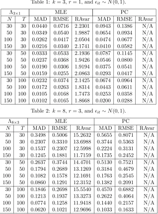
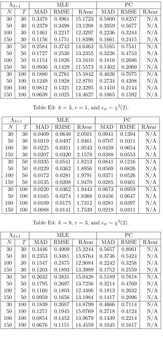
Throughout this section, we assume that the number of common factors is known. There are a number of methods at hand to determine the number of factors, for exam-ple, the information criterion method by Bai and Ng (2002), the largest eigenvalue-ratios method by Ahn and Horenstein (2013) and the eigenvalue empirical distribution method by Onatski (2010). If the number of factors is unknown, one can choose any of the method mentioned above to estimate it. Tables 1 and 2 present the performance of the MLE and the PC estimate for normal errors under the sample sizes ofN = 30,50,100,150and T = 30,50,100. The results under student-t errors and chi-square errors are almost the same as those for normal errors and are given in Table E1-E4 in the supplementary ap-pendix E (available upon request) to save space. All these results are obtained based on 1000 repetitions.
performs better than the PC estimate. Regarding the RAvar④
[image:21.612.148.466.198.628.2], we see that the MLE has almost constant RAvars when the time dimension T or the cross section dimension N increases, implying that the convergence rate of the MLE is √N T. This simulation result is consistent with our theoretical results in Section 4. In addition, it seems that the PC estimate also has √N T convergence rate from simulations. Finally, we note that the RMSEs of the MLE are smaller than those of the PC estimates, indicating that the MLE is more efficient than the PC estimates.
Table 1: k= 3,r = 1, and ϵit∼N(0,1).
Λ3×1 MLE PC
N T MAD RMSE RAvar MAD RMSE RAvar 30 30 0.0440 0.0716 2.2301 0.0943 0.1386 N/A 50 30 0.0349 0.0540 1.9887 0.0654 0.0934 N/A 100 30 0.0262 0.0417 2.0504 0.0474 0.0677 N/A 150 30 0.0216 0.0340 2.1741 0.0410 0.0582 N/A 30 50 0.0333 0.0533 2.1936 0.0787 0.1145 N/A 50 50 0.0237 0.0368 1.9426 0.0546 0.0800 N/A 100 50 0.0190 0.0306 1.9194 0.0375 0.0541 N/A 150 50 0.0159 0.0255 2.0863 0.0293 0.0417 N/A 30 100 0.0232 0.0374 2.1425 0.0674 0.0964 N/A 50 100 0.0172 0.0263 1.8314 0.0443 0.0611 N/A 100 100 0.0105 0.0168 1.7473 0.0253 0.0358 N/A 150 100 0.0102 0.0165 1.8668 0.0200 0.0288 N/A
Table 2: k= 8,r = 3, and ϵit∼N(0,1).
Λ8×3 MLE PC
N T MAD RMSE RAvar MAD RMSE RAvar 30 30 0.3498 0.5006 15.2632 0.5655 0.8071 N/A 50 30 0.2307 0.3310 13.6988 0.3744 0.5363 N/A 100 30 0.1537 0.2307 12.5998 0.2224 0.3131 N/A 150 30 0.1245 0.1881 11.7159 0.1735 0.2452 N/A 30 50 0.2637 0.3744 14.4701 0.5130 0.7521 N/A 50 50 0.1794 0.2689 13.1269 0.3184 0.4679 N/A 100 50 0.1082 0.1578 12.1691 0.1763 0.2545 N/A 150 50 0.0860 0.1291 12.3152 0.1382 0.2091 N/A 30 100 0.1846 0.2698 15.5540 0.4570 0.6882 N/A 50 100 0.1213 0.1937 13.3273 0.2622 0.4064 N/A 100 100 0.0774 0.1258 11.9418 0.1440 0.2157 N/A 150 100 0.0620 0.1021 12.9696 0.1033 0.1633 N/A
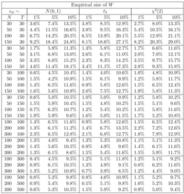
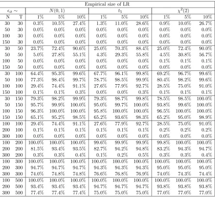
8.2 Empirical size of the W test
In this subsection, we use simulations to study the empirical size of theW statistic. The data generating process is the same as in previous subsection, but with more combinations
④
of (N, T). We investigate the performance of W under three nominal levels 1%, 5% and 10%. The empirical sizes of W for the case (k, r) = (3,1) are given in Table 3, which is obtained from 1000 repetitions.
Table 3: The empirical size of the test statisticW for(k, r) = (3,1)
Empirical size ofW
ϵit∼ N(0,1) t5 χ2(2)
N T 1% 5% 10% 1% 5% 10% 1% 5% 10%
30 30 3.6% 7.4% 13.5% 3.8% 8.5% 12.9% 2.7% 8.0% 13.3%
50 30 4.4% 11.5% 16.6% 3.9% 9.5% 16.3% 5.4% 10.5% 16.1% 100 30 6.7% 14.2% 20.5% 6.5% 13.9% 20.1% 5.5% 12.9% 21.1% 150 30 9.2% 18.4% 24.8% 8.1% 18.6% 27.1% 8.2% 20.3% 29.0%
30 50 1.7% 5.9% 11.3% 1.3% 5.8% 12.7% 1.7% 6.6% 11.6%
50 50 3.1% 6.8% 13.0% 2.6% 6.1% 11.0% 2.0% 7.0% 12.1%
100 50 3.3% 8.0% 15.2% 2.3% 8.3% 14.2% 3.5% 9.7% 15.7%
150 50 4.6% 11.4% 18.1% 3.4% 11.1% 17.3% 2.8% 9.3% 15.8% 30 100 0.6% 4.5% 10.4% 1.4% 4.0% 10.6% 1.0% 4.8% 10.9%
50 100 1.5% 4.2% 10.9% 1.5% 6.1% 9.9% 1.2% 5.8% 11.7%
100 100 1.4% 6.5% 11.6% 0.9% 5.8% 12.6% 1.5% 6.5% 12.4% 150 100 1.6% 5.6% 10.9% 2.0% 7.5% 12.7% 1.9% 5.8% 11.3%
30 150 0.6% 5.0% 10.5% 1.0% 5.0% 9.9% 1.2% 5.8% 10.2%
50 150 1.5% 5.9% 10.4% 1.5% 4.8% 10.2% 1.5% 5.1% 9.6%
100 150 0.7% 6.2% 10.7% 1.2% 5.4% 10.2% 1.5% 5.8% 11.6%
150 150 1.9% 5.9% 9.6% 1.6% 5.0% 11.5% 1.7% 5.2% 10.8%
100 100 1.4% 6.5% 11.6% 0.9% 5.8% 12.6% 1.5% 6.5% 12.4% 200 100 1.3% 6.1% 11.2% 1.4% 6.7% 13.5% 2.2% 7.2% 12.6% 300 100 2.3% 6.5% 12.8% 2.1% 6.8% 12.7% 1.8% 7.9% 12.9%
100 200 1.3% 4.0% 9.4% 1.3% 5.3% 10.8% 1.1% 5.1% 11.3%
200 200 1.4% 5.6% 10.5% 0.9% 4.9% 9.6% 1.4% 6.1% 11.6%
300 200 1.3% 6.1% 8.6% 1.5% 5.4% 11.6% 1.5% 5.9% 11.7%
100 300 0.4% 4.5% 9.5% 1.2% 5.1% 11.8% 1.2% 5.1% 9.2%
200 300 0.9% 6.1% 10.5% 1.3% 4.9% 9.1% 0.8% 6.2% 11.6%
300 300 1.3% 5.2% 10.9% 0.7% 3.9% 8.5% 1.2% 4.4% 9.0%
100 500 0.8% 5.3% 9.8% 0.8% 4.6% 10.9% 1.1% 5.2% 9.7%
200 500 0.9% 5.4% 9.8% 0.5% 5.1% 9.8% 1.0% 5.2% 10.3%
300 500 0.6% 5.3% 10.5% 1.5% 5.9% 9.2% 0.9% 5.0% 9.4%
From the results in Table 3, we emphasize the following findings. First, the performance of the W test is considerably good overall. Except for the sample size when T is small, almost all the empirical sizes of the W statistic fall in the interval [5%,10%] under the 5% nominal level. Second, the distribution type of errors has no significant impact on the performance of W. The W statistic performs very similarly under three different error distributions. This is consistent with the theoretical result in Section 5. Third, the performance ofW is closely linked with time period numberT, loosely with the number of unitsN. For example, whenT = 30, theW statistic suffers a mildly severe size distortion. But whenT grows to 50, the size distortion considerably decreases. As regard to N, we see that the W statistic performs well even when N = 30. We conjecture the reason is that when T is small, the variance σ2
i are estimated inaccurately, which leads to a poor