An Empirical Study of Smoothing Techniques for Language Modeling

(1)

An Empirical Study of Smoothing Techniques for Language

Modeling

S t a n l e y

F . C h e n H a r v a r d U n i v e r s i t y A i k e n C o m p u t a t i o n L a b o r a t o r y

33 O x f o r d S t . C a m b r i d g e , M A 0 2 1 3 8

sfc©eecs, harvard, edu

J o s h u a G o o d m a n

H a r v a r d U n i v e r s i t y A i k e n C o m p u t a t i o n L a b o r a t o r y

33 O x f o r d S t . C a m b r i d g e , M A 0 2 1 3 8

goodma.n~eecs, h a r v a r d , edu

A b s t r a c t

We present an extensive empirical comparison of several smoothing techniques in the domain of language modeling, including those described by Jelinek and Mer- cer (1980), Katz (1987), and Church and Gale (1991). We investigate for the first time how factors such as training d a t a

size, corpus

(e.g.,

Brown versus Wall Street

Journal), and n-gram order (bigram versus trigram) affect the relative performance of these methods, which we measure through the cross-entropy of test data. In addition, we introduce two novel smoothing techniques, one a variation of Jelinek-Mercer smoothing and one a very simple linear interpolation technique, both of which out- perform existing methods.

1

I n t r o d u c t i o n

Smoothing

is a technique essential in the construc- tion of n-gram language models, a staple in speech recognition (Bahl, Jelinek, and Mercer, 1983) as well as m a n y other domains (Church, 1988; Brown et al.,

1990; Kernighan, Church, and Gale, 1990). A

lan-

guage model

is a probability distribution over strings

P(s)

that a t t e m p t s to reflect the frequency with which each string s occurs as a sentence in natural text. Language models are used in speech recognition to resolve acoustically ambiguous utterances.

For example, if we have that

P(it takes two)

>>

P(it takes too),

then we know

ceteris paribus

to pre- fer the former transcription over the latter.

While smoothing is a central issue in language modeling, the literature lacks a definitive comparison between the many existing techniques. Previ- ous studies (Nadas, 1984; Katz, 1987; Church and Gale, 1991; MacKay and Peto, 1995) only compare a small number of methods (typically two) on a single corpus and using a single training data size. As a result, it is currently difficult for a researcher to intelligently choose between smoothing schemes.

In this work, we carry out an extensive

empirical comparison of the most widely used smoothing techniques, including those described by 3elinek and Mercer (1980), Katz (1987), and Church and Gale (1991). We carry out experiments

over m a n y training d a t a sizes on varied corpora

us-

ing

both bigram and trigram models. We demon-

strate that the relative performance of techniques depends greatly on training d a t a size and n-gram order. For example, for bigram models produced from large training sets Church-Gale smoothing has superior performance, while Katz smoothing performs best on bigram models produced from smaller data. For the methods with parameters t h a t can be tuned to improve performance, we perform an a u t o m a t e d search for optimal values and show t h a t sub-optimal parameter selection can significantly de- crease performance. To our knowledge, this is the first smoothing work that systematically investigates any of these issues.

In addition, we introduce two novel smoothing techniques: the first belonging to the class of smoothing models described by 3elinek and Mer- cer, the second a very simple linear interpolation

method. While being relatively simple to imple-

ment, we show that these methods yield good performance in bigram models and superior performance in trigram models.

We take the performance of a m e t h o d m to be its cross-entropy on test data

1 IT

I v T - log

Pro(t,)

i = 1

where

Pm(ti)

denotes the language model produced

with m e t h o d m and where the test d a t a T is com- posed of sentences ( t l , . . . , t z r ) and contains a total

of

NT

words. The entropy is inversely related to

the average probability a model assigns to sentences in the test data, and it is generally assumed that lower entropy correlates with better performance in applications.

(2)

1.1 S m o o t h i n g n - g r a m M o d e l s

In n - g r a m language modeling, the probability of a

string P ( s ) is expressed as the product of the prob-

abilities of the words t h a t compose the string, with each word probability conditional on the identity of

the last n - 1 words, i.e., i f s = w l - . . w t we have

l 1

P ( s ) = H P(wi[w{-1) ~ 1-~ P i-1

(1)

i=1 i=1

where w i j denotes the words wi • •. wj. Typically, n is

taken to be two or three, corresponding to a bigram

or trigram model, respectively. 1

Consider the case n = 2. To estimate the proba-

bilities P ( w i l w i - , ) in equation (1), one can acquire

a large corpus of text, which we refer to as training

data, and take

P(Wi-lWi)

PML(Wil i-1) --

P(wi-1)

c(wi-lWi)/Ns

e(wi-1)/Ns

c(wi_ w )

where c(c 0 denotes the n u m b e r of times the string

c~ occurs in the text and N s denotes the total num-

ber of words. This is called the maximum likelihood

(ML) e s t i m a t e for P ( w i l w i _ l ) .

While intuitive, the m a x i m u m likelihood estimate is a poor one when the a m o u n t of training d a t a is small c o m p a r e d to the size of the model being built, as is generally the case in language modeling. For example, consider the situation where a pair of words,

or bigram, say burnish the, doesn't occur in the

training data. Then, we have PML(the Iburnish) = O,

which is clearly inaccurate as this probability should be larger t h a n zero. A zero bigram probability can lead to errors in speech recognition, as it disallows the b i g r a m regardless of how informative the acous-

tic signal is. T h e t e r m smoothing describes tech-

niques for adjusting the m a x i m u m likelihood esti- m a t e to hopefully produce more accurate probabilities.

As an example, one simple s m o o t h i n g technique is to pretend each b i g r a m occurs once more than it ac- tually did (Lidstone, 1920; Johnson, 1932; Jeffreys, 1948), yielding

C(Wi-lWi) "[- 1

= + IVl

where V is the vocabulary, the set of all words be-

ing considered. This has the desirable quality of

1 T o m a k e t h e t e r m P(wdw[Z~,,+~) m e a n i n g f u l for i < n , o n e c a n p a d t h e b e g i n n i n g o f t h e s t r i n g w i t h a d i s t i n g u i s h e d t o k e n . I n t h i s w o r k , we a s s u m e t h e r e a r e n - 1 s u c h d i s t i n g u i s h e d t o k e n s p r e c e d i n g e a c h s e n t e n c e .

preventing zero b i g r a m probabilities. However, this scheme has the flaw of assigning the s a m e probabil-

ity to say, burnish the and burnish thou (assuming

neither occurred in the training data), even though intuitively the former seems more likely because the

word the is much more c o m m o n than thou.

To address this, another smoothing technique is to

interpolate the bigram model with a u n i g r a m model

PML(Wi) = c ( w i ) / N s , a model t h a t reflects how of-

ten each word occurs in the training data. For example, we can take

Pinto p( i J i-1) = APM (w pW _l) + (1 -

getting the behavior that bigrams involving c o m m o n words are assigned higher probabilities (Jelinek and Mercer, 1980).

2 P r e v i o u s W o r k

T h e simplest type of smoothing used in practice is

additive smoothing (Lidstone, 1920; Johnson, 1932;

aeffreys, 1948), where we take

i

w i-1 ₌ e ( w i _ , , + l ) +

+ elVl

(2)

and where Lidstone and Jeffreys advocate /i = 1. Gale and Church (1990; 1994) have argued t h a t this m e t h o d generally performs poorly.

The Good-Turing estimate (Good, 1953) is central to m a n y smoothing techniques. It is not used directly for n - g r a m smoothing because, like additive smoothing, it does not perform the interpolation of lower- and higher-order models essential for good performance. G o o d - T u r i n g states t h a t an n - g r a m t h a t occurs r times should be treated as if it had occurred r* times, where

r* = (r + 1)n~+l

and where n~ is the n u m b e r of n - g r a m s that. occur exactly r times in the training data.

Katz smoothing (1987) extends the intuitions of Good-Turing by adding the interpolation of higher- order models with lower-order models. It is perhaps the most widely used smoothing technique in speech recognition.

Church and Gale (1991) describe a smoothing m e t h o d that combines the G o o d - T u r i n g estimate

with bucketing, the technique of partitioning a set,

of n - g r a m s into disjoint groups, where each group is characterized independently through a set of parameters. Like Katz, models are defined recursively in terms of lower-order models. Each n - g r a m is assigned to one of several buckets based on its fre-

quency predicted from lower-order models. Each

(3)

N d b u c k e t i n g

2

° * ~ ° % °

o °$ o • .

° . ~ °e o * ° * ° * ° • ** o ~ , ~ L . s °o . • o

oO o ~ o ° *b

; . ° * ~ a - : . . • . °

• % a t

...,~;e.T¢:

° . . . : °

° % o % * * ° ~ - °

~ ° ~ ° o o

° ° • ° ~ °

o *

° o

o o

, , , i , , , i , , , i , " . . . . 0

l o 1 0 0 1 0 0 0 1 0 0 0 0 1 0 0 0 0 0 0 . o 0 1

r~rn~¢ o f c o u n t s i n d i s t N ~ t ] o n

n e w b u c k e t i n g

. , . . . ,

oeW~ o

. 6 ' V ,

* ° N a , o

* * I * , , I , , * I , , * I , * 0 . 0 1 0 . 1 1 1 0

a v e r a g e r ~ n - z e m c o u n t i n d i s ~ b u t i o n r ~ n u s O n e

Figure 1: )~ values for old and new bucketing schemes for Jelinek-Mercer smoothing; each point represents a single bucket

T h e other s m o o t h i n g technique besides Katz s m o o t h i n g widely used in speech recognition is due to Jelinek and Mercer (1980). T h e y present a class of s m o o t h i n g models t h a t involve linear interpola-

tion,

e.g.,

Brown et al. (1992) take

i - - 1

PML(Wi IWi-n+l) "Iv

~ W i _ _ 1 i - - 1

i - - n - ] - I

P~ / W i - 1 ,

( 1 - - )~to~-~ ) inte~pt

i wi_n+2)

(3)

i - - u - I - 1

T h a t is, the m a x i m u m likelihood estimate is inter- polated with the s m o o t h e d lower-order distribution, which is defined analogously. Training a distinct

I ~-1 for each

wi_,~+li-1

is not generally felicitous;

W i - - n - { - 1

Bahl, Jelinek, and Mercer (1983) suggest partition-

i - 1

ing the 1~,~-~ into buckets according to

c(wi_~+l),

i - - n - l - 1

where all )~w~-~ in the same bucket are constrained

i - - n - l - 1

to have the s a m e value.

To yield meaningful results, the d a t a used to esti-

m a t e the A~!-, need to be disjoint from the d a t a

~-- n"l-1

used to calculate PML .2 In

held-out interpolation,

one reserves a section of the training d a t a for this purpose. Alternatively, aelinek and Mercer describe

a technique called

deleted interpolation

where differ-

ent parts of the training d a t a rotate in training either

PML or the A,o!-' ; the results are then averaged.

z-- n - [ - I

Several s m o o t h i n g techniques are m o t i v a t e d

within a Bayesian framework, including work by Nadas (1984) and M a c K a y and Peto (1995).

3

Novel S m o o t h i n g Techniques

Of the great m a n y novel m e t h o d s t h a t we have tried, two techniques have performed especially well.

2When the same data is used to estimate both, setting

all )~ ~-~ to one yields the optimal result.

W l - - n - l - 1

3.1 M e t h o d

average-count

This scheme is an instance of Jelinek-Mercer smoothing. Referring to equation (3), recall t h a t

Bahl et al. suggest bucketing the A~!-I according

i - - 1

to c(Wi_n+l). We have found t h a t partitioning the

~ ! - ~ according to the average n u m b e r of counts

* - - ~ + 1

per non-zero element ~(~--~"+1) yields better

I w i : ~ ( ~ : _ . + ~ ) > 0 1

results.

Intuitively, the less sparse the d a t a for e s t i m a t - ing

PML(WilWi_n+l),

i-1 _{the larger A~,~-~ should be.}

*-- ~-t-1

While larger

c(wi_n+l)

i-1 generally correspond to less

sparse distributions, this quantity ignores the allo- cation of counts between words. For example, we would consider a distribution with ten counts distributed evenly a m o n g ten words to be much more sparse t h a n a distribution with ten counts all on a single word. T h e average n u m b e r of counts per word seems to more directly express the concept of sparse- ness,

In Figure 1, we graph the value of ~ assigned to each bucket under the original and new bucketing schemes on identical data. Notice t h a t the new bucketing scheme results in a much tighter plot, indicat- ing t h a t it is better at grouping together distributions with similar behavior.

3.2 M e t h o d

one-count

This technique combines two intuitions. First,

MacKay and Peto (1995) argue t h a t a reasonable form for a smoothed distribution is

• i - 1

Pone(W i i-1

c(wL, +l) + Po,,e(wilw _ +9

I W i - - n q - 1 ) = i - - 1

c(wi_n+l) +

T h e p a r a m e t e r a can be thought of as the number of counts being added to the given distribution,

[image:3.612.88.538.82.240.2]

(4)

where the new counts are distributed as in the lower- order distribution. Secondly, the Good-Turing esti- m a t e can be interpreted as stating t h a t the n u m b e r of these extra counts should be proportional to the n u m b e r of words with exactly one count in the given distribution. We have found t h a t taking

i - 1

O~ = "y [ n l ( W i _ n + l ) -~- ~] ( 4 )

works well, where

i - i i

is the n u m b e r of words with one count, and where/3 and 7 are constants.

4 E x p e r i m e n t a l M e t h o d o l o g y

4.1 D a t a

We used the Penn treebauk and T I P S T E R cor- p o r a distributed by the Linguistic D a t a Consor- tium. From the treebank, we extracted text from the tagged Brown corpus, yielding about one million words. From T I P S T E R , we used the Associ- ated Press (AP), Wall Street Journal (WSJ), and San Jose Mercury News (SJM) data, yielding 123, 84, and 43 million words respectively. We created two distinct vocabularies, one for the Brown corpus and one for the T I P S T E R data. T h e former vocabulary contains all 53,850 words occurring in Brown; the latter vocabulary consists of the 65,173 words occurring at least 70 times in T I P S T E R .

For each experiment, we selected three segments of held-out d a t a along with the segment of train-

ing data. One held-out segment was used as the

test d a t a for performance evaluation, and the other two were used as development test d a t a for opti- mizing the p a r a m e t e r s of each smoothing method. Each piece of held-out d a t a was chosen to be roughly 50,000 words. This decision does not reflect practice very well, as when the training d a t a size is less than 50,000 words it is not realistic to have so much devel- o p m e n t test d a t a available. However, we m a d e this decision to prevent us having to optimize the training versus held-out d a t a tradeoff for each d a t a size. In addition, the development test d a t a is used to optimize typically very few parameters, so in practice small held-out sets are generally adequate, and perhaps can be avoided altogether with techniques such as deleted estimation.

4.2 S m o o t h i n g I m p l e m e n t a t i o n s

In this section, we discuss the details of our imple- m e n t a t i o n s of various smoothing techniques. Due to space limitations, these descriptions are not com- prehensive; a more complete discussion is presented in Chen (1996). T h e titles of the following sections include the m n e m o n i c we use to refer to the imple- m e n t a t i o n s in later sections. Unless otherwise speci- fied, for those s m o o t h i n g models defined recursively in terms of lower-order models, we end the recursion

by taking the n = 0 distribution to be the uniform

distribution Punif(wi) = l / I V [ . For each m e t h o d , we

highlight the p a r a m e t e r s (e.g., Am and 5 below) t h a t

can be tuned to optimize performance. P a r a m e t e r values are determined through training on held-out data.

4.2.1 B a s e l i n e S m o o t h i n g ( i n t e r p - b a s e l i n e )

For our baseline smoothing m e t h o d , we use an instance of Jelinek-Mercer smoothing where we con-

strain all A,~!-I to be equal to a single value A,~ for

, - n-hi

each n, i.e.,

i--1 i - 1

Pb so(wilw _ +i) = A,, +

(I

--

Am)

Pbase(WilWi_n+2)

4.2.2 A d d i t i v e S m o o t h i n g ( p l u s - o n e a n d

plus-delta)

We consider two versions of additive smoothing. Referring to equation (2), we fix 5 = 1 in p l u s - o n e smoothing. In p l u s - d e l t a , we consider any 6.

4.2.3 K a t z S m o o t h i n g ( k a t z )

While the original paper (Katz, 1987) uses a single p a r a m e t e r k, we instead use a different k for each n > 1, k,~. We s m o o t h the u n i g r a m distribution using additive smoothing with p a r a m e t e r 5.

4.2.4 C h u r c h - G a l e S m o o t h i n g

(church-gale)

To s m o o t h the counts n~ needed for the Good- Turing estimate, we use the technique described by Gale and Sampson (1995). We s m o o t h the unigram distribution using Good-tiering without any bucketing.

Instead of the bucketing scheme described in the original paper, we use a scheme analogous to the one described by Bahl, Jelinek, and Mercer (1983). We make the assumption t h a t whether a bucket is large enough for accurate G o o d - T u r i n g estimation depends on how m a n y n - g r a m s with non-zero counts occur in it. Thus, instead of partitioning the space

of P ( w i - J P ( w i ) values in some uniform way as was

done by Church and Gale, we partition the space so t h a t at least Cmi n non-zero n - g r a m s fall in each bucket.

Finally, the original paper describes only bigram smoothing in detail; extending this m e t h o d to tri- g r a m smoothing is ambiguous. In particular, it is unclear whether to bucket trigrams according to

i - 1 i--1

P ( w i _ J P ( w d or P ( w i _ J P ( w i l w i - 1 ) . We chose the

former; while the latter m a y yield better performance, our belief is t h a t it is much more difficult to implement and t h a t it requires a great deal more computation.

4.2.5 J e l i n e k - M e r c e r S m o o t h i n g

(interp-held-out and interp-del-int)

We implemented two versions of Jelinek-Mercer smoothing differing only in what d a t a is used to

(5)

train the A's. We bucket the A ~-1 according to

Wi--n-bl i-1

C(Wi_~+I) as suggested by Bahl et al. Similar to our

Church-Gale implementation, we choose buckets to ensure that at least Cmi n words in the data used to train the A's fall in each bucket.

In i n t e r p - h e l d - o u t , the A's are trained using held-out interpolation on one of the development

test sets. In i n t e r p - d e l - i n t , the A's are trained

using the relaxed deleted interpolation technique de-

scribed by Jelinek and Mercer, where one word is

deleted at a time. In i n t e r p - d e l - i n t , we bucket

an n - g r a m according to its count before deletion, as this turned out to significantly improve performance.

4.2.6 N o v e l S m o o t h i n g M e t h o d s

(new-avg-count and new-one-count)

The implementation n e w - a v g - c o u n t , correspond-

ing to smoothing m e t h o d average-count, is identical

to i n t e r p - h e l d - o u t except that we use the novel bucketing scheme described in section 3.1. In the implementation n e w - o n e - c o u n t , we have different parameters j3~ and 7~ in equation (4) for each n.

5 R e s u l t s

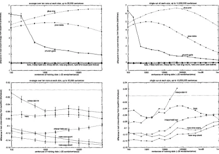
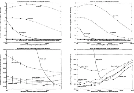
In Figure 2, we display the performance of the i n t e r p - b a s e l i n e m e t h o d for bigram and trigram models on T I P S T E R , Brown, and the WSJ subset of T I P S T E R . In Figures 3-6, we display the relative performance of various smoothing techniques with respect to the baseline method on these corpora, as measured by difference in entropy. In the graphs on the left of Figures 2-4, each point represents an average over ten runs; the error bars represent the empirical standard deviation over these runs. Due to resource limitations, we only performed multiple runs for d a t a sets of 50,000 sentences or less. Each point on the graphs on the right represents a single run, but we consider sizes up to the amount of d a t a available. The graphs on the b o t t o m of Fig- ures 3-4 are close-ups of the graphs above, focusing on those algorithms that perform better than the baseline. To give an idea of how these cross-entropy differences translate to perplexity, each 0.014 bits correspond roughly to a 1% change in perplexity.

In each run except as noted below, optimal values for the parameters of the given technique were searched for using Powell's search algorithm as real-

ized in Numerical Recipes in C (Press et al., 1988,

pp. 309-317). Parameters were chosen to optimize the cross-entropy of one of the development test sets associated with the given training set. To constrain the search, we searched only those parameters that were found to affect performance significantly, as verified through preliminary experiments over several data sizes. For k a t z and c h u r c h - g a l e , we did not perform the parameter search for training sets over 50,000 sentences due to resource constraints, and instead manually extrapolated parameter val-

Method Lines

interp-baseline ~ 400

plus-one 40

p l u s - d e l t a 40

k a t z 300

church-gale i000

±nterp-held-out 400

interp-del-int 400

new-avg-count 400

new-one-count 50

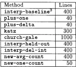
Table 1: Implementation difficulty of various methods in terms of lines of C + + code

ues from optimal values found on smaller d a t a sizes. We ran i n t e r p - d e l - i n t only on sizes up to 50,000 sentences due to time constraints.

From these graphs, we see that additive smoothing performs poorly and that methods k a t z and

i n t e r p - h e l d - o u t consistently perform well. Our

implementation c h u r c h - g a l e performs poorly except on large bigram training sets, where it performs the best. The novel methods n e w - a v g - c o u n t and n e w - o n e - c o u n t perform well uniformly across training data sizes, and are superior for trigram models. Notice that while performance is relatively consis- tent across corpora, it varies widely with respect to training set size and n - g r a m order.

The method interp-del-int performs signifi-

cantly worse than i n t e r p - h e l d - o u t , though they differ only in the d a t a used to train the A's. However, we delete one word at a time in i n t e r p - d e l - i n t ; we hypothesize that deleting larger chunks would lead to more similar performance.

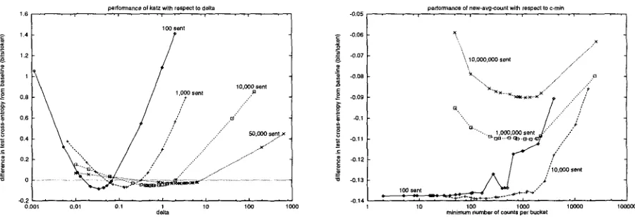
In Figure 7, we show how the values of the parameters 6 and Cmin affect the performance of methods k a t z and n e w - a v g - c o u n t , respectively, over several training d a t a sizes. Notice that poor parameter setting can lead to very significant losses in performance, and that optimal parameter settings depend on training set size.

To give an informal estimate of the difficulty of implementation of each method, in Table 1 we display the number of lines of C + + code in each implementation excluding the core code c o m m o n across techniques.

6 D i s c u s s i o n

To our knowledge, this is the first empirical comparison of smoothing techniques in language modeling of such scope: no other study has used multiple training data sizes, corpora, or has performed parameter optimization. We show that in order to completely

3To implement the baseline method, we just used the i n t e r p - h e l d - o u t code as it is a special case. Written anew, it probably would have been about 50 lines.

[image:5.612.361.493.76.193.2]

(6)

11.5

10.5

10

9.5

0

a.5

average over ten runs at each size, up to 50,0OO sentences

" - ~ : : : . TIPSTER bigram " - . "'~:-WS.J bigrarn

1000 10000 sentences of training data (-25 words~sentence)

t l . 5 11 10.5 tO 9.5 0 8.5 8 7.5 7 6.5 tOO

single run at each size

",..

~io~n t rigrarn

-.~ ~...

" ' , . , " ' " ~ ' . : " - ~ . TIPSTER bigram

. . . , . . : = : : : : ; . . .

V~SJ b~gram . TIPSTER tdgra~

tO00 1O000 100000 le+06 )e+07 sentences of training data (-25 words/sentence)

Figure 2: Baseline cross-entropy on test data; graph on left displays averages over ten runs for training sets up to 50,000 sentences, graph on right displays single runs for training sets up to 10,000,000 sentences

average over ten runs at each size, up to 50,000 sentences 7 . . . , . . . ) • . .

l~Us-one ... ~ ... ~ ... = ... 6 ... ~ ...

c~ ... plu s=dsita ... I ....

4 ... ..

!

._c

- t .. ... ... ~ ... ... .. ~

1000 10000 sentences of training data (-25 wordS/sentence)

single run at each size, up to 10,000,000 sentences

. . , . . , . . . , . . . , . .

+ ... +....--~ plus~ne

... ..~...y~ " ' " ' ~ " -..+.,..,,., .,-" .... o.-..-~'""~...~ ' - . . .

--.. ~ ,

2=,j ...

...

1 J .church-gata " " *

ks/z, interp-held-out, ~nterpdel-int, new-avg-count, new-one-count (see below)

- 1 , • . . . . . . . . ' ' ' " ' "

100 1000 10000 100000 le+06 le+07 sentences of training data (-25 words~sentence)

average over ten runs at each size, up to 50,000 sentences single run at each size, Up to 10,000,000 sentences 0.04 . . , • - - , • - , - - , •

0 ...

-0,02 " ~ " - . . i n t e r p - d e l q n t

-0.00

~.1 n ...

[image:6.612.79.526.93.252.2] [image:6.612.78.523.330.644.2]

... ~ t 1 ... ~ ... ~ ...

... ~ ... ::::::::::::::::::::::::::::::::::::::::::::::

- 0 . 1 6 . .... ... J . . . .

too 1000 10000

sentences of training data (-25 words~sentence}

o.02 o .,';'~o~o,-~nt t

-0.02

-0.04 ~.-..._Z .~ . . . ~ . - . katz d

I

" / : * " -'-"(" '" " ' m .

. . . ~ . , ] [ F ,.a ... a " " ~ ' ,

JO.O8 " inteq)qle)d-out . . o ' " "

~3.1 .~" . ~ - - - - ~ . new-one-count c / " x . . . - ~

-0.12 ... " t ~ " " " " . . . ~ - . . . - " . / new-svg-count

- 0 . 1 4 k . . . x _ ~ _ . . _ ~ . . . i " "~"~ "0.1610 o

lO0O 1OOOO 10oooo le+06 le+07 sentences of training data (-25 words/sentonce)

Figure 3: Trigram model on T I P S T E R data; relative performance of various m e t h o d s with respect to baseline; graphs on left display averages over ten runs for training sets up to 50,000 sentences, graphs on right display single runs for training sets up to 10,000,000 sentences; top graphs show all algorithms, b o t t o m graphs z o o m in on those m e t h o d s that perform better than the baseline m e t h o d

(7)

E

=o

average over ten runs at each size, up to 50,000 senlences

5 . . . , . . . , • • - 4.6 .... ~- ... "~'" plus-o'n~ ... ~ ....

4 ...

3.S "

3 ... t~.,, " " - ~ ... ~ p l u s 4 e l ~

2.5 ... *

1. I

church*gale '

0 . 5

0 . . . . .

- 0 5

100 1000 10000

sentences of training data ( - 2 6 words/sentence) average over t ~ runs at each size, u p to 50,000 sentences 0.02 . . . , . . . , . . •

-0.02 " " "~... humh*gale

~- ... ...~ ... {. ... -0.00

... ~ . . . - ' ~ - ' ~ " :=L::~" T n : w : n 2 o u n t / ~ . . . 1

.0.14

100 1000 10000

sentences of training data ( - 2 6 words/sentence)

single run at each size, up to 10,000,000 sentences

5 , • . , . • . . . , . • . , . •

4 " ..

3 . 5 "~"'~"... I~US*one

2.5 t ' ' ° ' " " ' ~ ' " " ' o . . . " " " o . " * .

1 f - -church-gale , ~ " "~" " "'~... p us-de ta O.5 " ~ - . .

- - . _ o .

~3.6 T , ,k~tz, taterp-he~-out., interp~, el~tat, ,~ew,~zvg~ou ' . . . ~ n e . ~ o u n t ! . . . ,ow), l 100 1000 10000 100000 l e + 0 6 l e + 0 7

sentences of training data ( - 2 6 words/sentence) stagle r~n at each size, up to 10,OCO,O00 sentences

0.02 • • • , . , • . , . , . . .

o I

-0.02 church*gale

...~:,'~

-0.04 ~ " " ,¢ " .. " . n erp-he d-out . " ~,~

- ~ Interprdel-mt . . - .* ~ ' "

... ~ . . ~ . ~ . / . - ~ 0 ~

-0.1 new-one-count ..~D -...B'" .~.. • . -..~ j . ~ . ~ . . : . : : ; $ . , ~Om 1 2

ew-avg-count

.0.14 ' , , I , , , i , , , m , . , I , , 10o 10oo 1ooo0 1oo000 l e + 0 6 l e + 0 7

sentences of training data (-25 wo~ds/sentence)

Figure 4: Bigram model on T I P S T E R data; relative performance of various methods with respect to baseline; graphs on left display averages over ten runs for training sets up to 50,000 sentences, graphs on right display single runs for training sets up to 10,000,000 sentences; top graphs show all algorithms, b o t t o m graphs zoom in on those methods that perform better than the baseline method

bigram model 0.02 . . . , . . . ,

0

i -0.02 church-gale

interprdel-int .0,04 ..-~, . . . ~. .0.00

.0.o8 . . . z " ... ~*..

-0.12 "= . ~inte~p~held-out

lew-a-~n~t...~--~272~::'z--.. " n ~ : o r p e - ~ t a ... D . . .

-0.16

-0.18 . . . i . . . i

100 1000 IOQO0

sentences of training data (-21 words~sentence)

tzigram model

0 ... .0.02

-0.06 katz . - - ~ " " ' ~ ' " ' " " ' " • .. - : : : . . . . . .,,<.:..-"

-0.06 .-" ... . . . i r ~ t e t p..<1 el-~ip_t .. . .

.0.12 :::.-.. " ' ~ = . . . . ... ~ ... Q.. interp*held-out

. . . 7~.=: =-P~::.... " ... e . . . o . . . e ... ~ ...

.0.14 - ~ - = ' : : : = * ~ - ~ _ . _ _ _ ~ new-one-count

- 0 . 1 6 0 0

1000 10000 sentences of traJelng data (-21 words/sentence)

Figure 5: Bigram and trigram models on Brown corpus; relative performance of various methods with respect to baseline

[image:7.612.86.537.100.413.2] [image:7.612.85.536.513.668.2]

(8)

bigram model tdgram m o d e l

"(,

~

. . .

o 0 i ~ 0 . 0 2

-0.02 hurch-gale

~ ' - - n t erp~J el-int " ~

-0.04 .. . . ~ -0.02

inte rp-d el-int " . . ~ inte rpheld~out . . . ~ " " ~ " ' - ~

E -0.06 • " . , ~ , ~ . ] ~ - . - ~,. " ' A . -- -0.06 . - ' - ' k a t z " " - ~ " - . = . .

-0°3 ' :i: , . . ... ::.>~,.- .~. ... . . ~ " ' - - : : : : . . ,

y

-oo i

-. . .

-0.14 • " " " "~ " • " -k-atz

-0.13 ~ -018 . . . = ' ' ,

1oo 1000 10oo0 100000 le+06 10o 1000 10000 100000 le+0o

sentences of training data ( - 2 5 words/sentence) sentences of t relelr~g data ( - 2 5 words/sentence)

Figure 6: Bigram and trigram models on Wall Street Journal corpus; relative performance of various methods with respect to baseline

z

~C

==

.=_

performance el katz with respect to delta

1.6 . . . . , • . . , . . , . . . , • . . , . . 10O senl

1.4 1.2

1

10,0O0 sent

0.8 1,0O0 sent ..a

0.6 / ' .,.~/" 0.4 / .-" .ED,O00 sent)<

0 . 2

" ' " ' d : . / .." ~ ' "

e . . . . I , , , i , , , r , , , I , , , i , , ,

0.0Ol o.01 0.1 1 lO 10o 1000

delta

-0.0O

-0.07

==-

-O.08

2 -0.O3

-0.1

-0.11

-0.12

-0.13

performance of new-avg-c~nt with respect to c-min

. . . , . . . , . .

x\

\ /

~'\ lO.000,000 sent _// "

/ " x \ , , .o

" , \ / / ,,,"

.... /

'"6. ..'"' 2 l

" " " ' u , 1 OO3,0OO s e n t " /

j / 1 0 , 0 O 0 sent

10 100 tO00 10(00 100000

minimum number of counts per bucket

Figure 7: Performance of katz and new-avg-count with respect to parameters ~ and Cmin, respectively

characterize the relative performance of two tech- niques, it is necessary to consider multiple training set sizes and to try both bigram and trigram mod- els. Multiple runs should be performed whenever possible to discover whether any calculated differ- ences are statistically significant. Furthermore, we show that sub-optimM parameter selection can also significantly affect relative performance.

We find that the two most widely used techniques, Katz smoothing and Jelinek-Mercer smoothing, per- form consistently well across training set sizes for both bigram and trigram models, with Katz smooth- ing performing better on trigram models produced from large training sets and on bigram models in general. These results question the generality of the previous reference result concerning Katz smooth- ing: Katz (1987) reported that his method slightly outperforms an unspecified version of Jelinek-Mercer smoothing on a single training set of 750,000 words. Furthermore, we show that Church-Gale smooth-

ing, which previously had not been compared with common smoothing techniques, outperforms all ex-

isting methods on bigram models produced from

large training sets. Finally, we find that our novel

methods average-count and one-count are superior

to existing methods for trigram models and perform

well on bigram models; method one-count yields

marginally worse performance but is extremely easy to implement.

In this study, we measure performance solely through the cross-entropy of test data; it would be interesting to see how these cross-entropy differ- ences correlate with performance in end applications such as speech recognition. In addition, it would be interesting to see whether these results extend to fields other than language modeling where smooth- ing is used, such as prepositional phrase attachment (Collins and Brooks, 1995), part-of-speech tagging (Church, 1988), and stochastic parsing (Magerman,

1994).

[image:8.612.77.523.80.237.2] [image:8.612.77.527.290.447.2]

(9)

Acknowledgements

The authors would like to thank Stuart Shieber and the anonymous reviewers for their comments on previous versions of this paper. We would also like to thank William Gale and Geoffrey Sampson for sup- plying us with code for "Good-Turing frequency estimation without tears." This research was supported by the National Science Foundation under Grant No. IRI-93-50192 and Grant No. CDA-94-01024. The second author was also supported by a National Sci- ence Foundation Graduate Student Fellowship.

References

Bahl, Lalit R., Frederick Jelinek, and Robert L. Mercer. 1983. A maximum likelihood approach

to continuous speech recognition. IEEE Trans-

actions on Pattern Analysis and Machine Intelli-

gence, PAMI-5(2):179-190, March.

Brown, Peter F., John Cocke, Stephen A. DellaPi- etra, Vincent J. DellaPietra, Frederick Jelinek, John D. Lafferty, Robert L. Mercer, and Paul S. Roossin. 1990. A statistical approach to machine

translation. Computational Linguistics, 16(2):79-

85, June.

Brown, Peter F., Stephen A. DellaPietra, Vincent J. DellaPietra, Jennifer C. Lai, and Robert L. Mer- cer. 1992. An estimate of an upper bound for

the entropy of English. Computational Linguis-

tics, 18(1):31-40, March.

Chen, Stanley F. 1996. Building Probabilistic Mod-

els for Natural Language. Ph.D. thesis, Harvard

University. In preparation.

Church, Kenneth. 1988. A stochastic parts program and noun phrase parser for unrestricted text. In Proceedings of the Second Conference on Applied

Natural Language Processing, pages 136-143.

Church, Kenneth W. and William A. Gale. 1991. A comparison of the enhanced Good-Turing and deleted estimation methods for estimating proba-

bilities of English bigrams. Computer Speech and

Language, 5:19-54.

Collins, Michael and James Brooks. 1995. Prepo- sitional phrase attachment through a backed-off model. In David Yarowsky and Kenneth Church,

editors, Proceedings of the Third Workshop on

Very Large Corpora, pages 27-38, Cambridge,

MA, June.

Gale, William A. and Kenneth W. Church. 1990. Estimation procedures for language context: poor

estimates are worse than none. In COMP-

STAT, Proceedings in Computational Statistics,

9th Symposium, pages 69-74, Dubrovnik, Yu-

goslavia, September.

Gale, William A. and Kenneth W. Church. 1994. What's wrong with adding one? In N. Oostdijk

and P. de Haan, editors, Corpus-Based Research

into Language. Rodolpi, Amsterdam.

Gale, William A. and Geoffrey Sampson. 1995.

Good-Turing frequency estimation without tears.

Journal of Quantitative Linguistics, 2(3). To ap-

pear.

Good, I.J. 1953. The population frequencies of

species and the estimation of population parame-

ters. Biometrika, 40(3 and 4):237-264.

Jeffreys, H. 1948. Theory of Probability. Clarendon

Press, Oxford, second edition.

Jelinek, Frederick and Robert L. Mercer. 1980. In- terpolated estimation of Markov source parame-

ters from sparse data. In Proceedings of the Work-

shop on Pattern Recognition in Practice, Amster-

dam, The Netherlands: North-Holland, May.

Johnson, W.E. 1932. Probability: deductive and

inductive problems. Mind, 41:421-423.

Katz, Slava M. 1987. Estimation of probabilities from sparse data for the language model com-

ponent of a speech recognizer. IEEE Transac-

tions on Acoustics, Speech and Signal Processing, ASSP-35(3):400-401, March.

Kernighan, M.D., K.W. Church, and W.A. Gale. 1990. A spelling correction program based on

a noisy channel model. In Proceedings of the

Thirteenth International Conference on Compu-

tational Linguistics, pages 205-210.

Lidstone, G.J. 1920. Note on the general case of the

Bayes-Laplace formula for inductive or a posteri-

ori probabilities. Transactions of the Faculty of

Actuaries, 8:182-192.

MacKay, David J. C. and Linda C. Peto. 1995. A hi-

erarchical Dirichlet language model. Natural Lan-

guage Engineering, 1(3):1-19.

Magerman, David M. 1994. Natural Language Pars-

ing as Statistical Pattern Recognition. Ph.D. the-

sis, Stanford University, February.

Nadas, Arthur. 1984. Estimation of probabilities in the language model of the IBM speech recognition

system. IEEE Transactions on Acoustics, Speech

and Signal Processing, ASSP-32(4):859-861, Au-

gust.

Press, W.H., B.P. Flannery, S.A. Teukolsky, and

W.T. Vetterling. 1988. Numerical Recipes in C.

Cambridge University Press, Cambridge.