CLIVAR Exchanges No 19 Decadal Variability and Predictability Part 1: Global aspects and the Atlantic sector

Exchanges No. 19

Decadal Variability and Predictability

Part 1: Global aspects and the Atlantic sector

Volume 6 No. 1

March 2001

Exchanges

Figure 1 from paper: PREDICATE: Mechanisms and Predictability of Decadal Fluctuations in At-lantic-European Climate by Rowan Sutton:

Observations of Northern European temperature anomalies (white line) and three forecasts demonstrating the large uncertainty in climate scenarios for the next 20 years. Note that the forecasts are not continuous with the observations because no information about the current ocean (and atmosphere) state is currently employed. This is a key issue that PREDICATE is addressing.

The paper appears on page 11.

As a result of the series of scientific workshops this and the next issue

of Exchanges highlight recent scientific work on the field of decdal

variability and predictability, one of the main streams of CLIVAR.

Uncertainty in current climate forecasts on decadal timescales

Northern European temperatures under three scenarios

4

2

0

-2

Editorial

Dear CLIVAR community,

One of the landmarks in climate research at the beginning of the 21st _{century is the progress that has been made in}

our understanding of decadal climate variability. 10 years ago, not much was known about the nature and the mecha-nisms of long-term climate variability. Improved model-ling techniques, progress in data analysis and new histori-cal and paleo data sets provide us with the basis to learn more about the long-term behaviour of our climate in the past and in future. Indeed, extending the climate record of paleo and instrumental data is one of CLIVAR’s objectives.

We still have a long way to go. There are substantial gaps in our knowledge, there are conflicting theories about the mechanisms of decadal variability and it is still debate-able to what extent relidebate-able long-term climate predictions will be possible within the next decade. Thus, the under-standing of decadal climate variability presents a big chal-lenge and CLIVAR is addressing it as one of the three main streams of the programme.

In CLIVAR’s Initial Implementation Plan the DecCen stream had five Principal Research Areas (PRA) dealing with the various aspects of decadal variability. Three con-cern phenomena in the Atlantic sector (North Atlantic Os-cillation, Tropical Atlantic Variability and Thermohaline Circulation) and these are being co-ordinated through the new CLIVAR Atlantic Panel. The scientific questions relat-ing to Pacific and Southern Ocean variability will be dealt with separately. CLIVAR panels for these two areas are currently being formed.

Underpinning this organizational structure, the sci-entific understanding of decadal variability has been docu-mented through a series of workshops that took place through autumn and winter 2000/2001. We reported in the last issue about three meetings: The workshops on “Decadal Predictability” and “Shallow Tropical/Subtropi-cal overturning cells and their interaction with the atmos-phere” and the “Southern Ocean Implementation Work-shop”. The WOCE/CLIVAR workshop on the representa-tiveness of the 1990s WOCE data set was reported on in the December 2000WOCE Newsletter (http:// www.woce.org).

Since then, three more meetings have taken place: the “Chapman Conference on the North Atlantic Oscilla-tion” undertook a comprehensive review of the progress in this area and workshops on Decadal Variability and on the implementation of CLIVAR in the Pacific were both held in Hawaii. Summaries from the NAO meeting and the Decadal Variability workshop can be found in this is-sue.

Our strategy with recent issues of CLIVAR Exchanges has been to go beyond the presentation of meeting summa-ries. We encouraged the submission of scientific results related to decadal variability and predictability and the response was very good. Thus, we were faced with either rejecting more than half of the submitted contributions or dedicating two issues of Exchanges to this topic. The qual-ity of the papers and the importance of the topic means we have taken the latter option. For this issue we grouped all the papers related to the Atlantic together with some more general topics. The next issue will focus on monsoons and Pacific decadal variability.

As we mentioned above, the organizational struc-ture of CLIVAR is expanding. Last year, the CLIVAR At-lantic panel and the VACS (Variability of the African Sys-tem) panel were formed. The Southern Ocean Workshop and the Pacific Implementation meeting recommended the establishment of oversight panels. It is expected that by end of 2001 the organizational structure of CLIVAR will be fully developed with panels and working groups that cover all aspects of the programme.

In contrast to this build-up, the resources of the ICPO are currently rather reduced following Fred Semazzi’s re-turn to the USA. This means a very high workload on the remaining ICPO staff such that some tasks can not be cov-ered adequately. For example we are currently not able to continue the development of the CLIVAR bibliography. This situation will improve very soon as we are in the proc-ess of hiring two new staff in addition to the recent recruit-ment of Carlos Ereño to cover VAMOS issues.

At the end of March the co-chairs of the CLIVAR SSG (Antonio Busalacchi and Juergen Willebrand) will present the annual summary of CLIVAR activities to the WCRP's Joint Scientific Committee (JSC) meeting in Boul-der. The JSC will particularly look for areas in which inter-actions between WCRP projects could be fruitful. CLIVAR is already developing strong links with ACSYS/CliC in the Southern Ocean and northern North Atlantic and with GEWEX on monsoon systems. We will report on the JSC meeting in the next issue.

We hope that you all enjoy this and the next issue of Exchanges documenting the progress in the field of decadal climate variability.

G.J. Boer

Canadian Centre for Climate Modelling and Analysis Atmospheric Environment Service

University of Victoria, Victoria, Canada [email protected]

Introduction

The analysis of decadal “potential predictability” in the coupled atmosphere-ocean system is, in essence, an analy-sis of long-timescale variability. Classical predictability measures the rate at which two initial close states of a sys-tem separate with time (and hence the rate of error growth in the system). Potential predictability, by contrast, is a measure of the variability of the system which attempts to quantify the fraction of long timescale variability that may be distinguished from the natural variability noise. This “signal”, if it exists and is of appreciable magnitude, is deemed to arise from physical processes operating in the system which are, at lease potentially, predictable.

Potential Predictability

We analyse the potential predictability of surface air tem-perature (SAT). The statistical approach generally follows Rowel (1998), and Rowell and Zwiers (1999) and assumes SAT variation is of the form T_ab = µ + s_a e_ab with µ the cli-mate mean, s_a the slow timescale “signal” component of the variability, and e_ab the remaining unpredictable climate noise. The ratio r = s_s2 _{/ (s}

s2 + se2) gives the fraction of the

total variance associated with the “potentially predictable” component. The value is tested against the null hypothesis that r = s_s2_{= 0. Model drift is first removed by fitting low}

order orthogonal polynomials in time at each point.

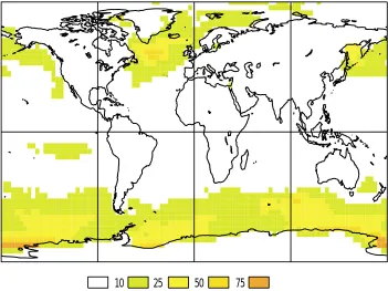
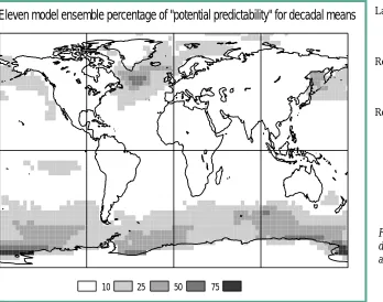
The result for the potential predictability of decadal means is shown in Figure 1. The result does not depend on a single model or simulation in this case but is an ensem-ble estimate of the potential predictability of the coupled system based on the control simulations of eleven models participating in the Coupled Model Intercomparison Project (see for example Meehl et al., 1997 and Lambert and Boer, 2001). The high latitude oceans are the dominant regions exhibiting potential predictability although there is some indication also in the tropical Pacific.

Discussion

The decadal predictability of the coupled atmosphere/ ocean/ice system is examined using a diagnostic “poten-tial predictability” approach. Preliminary results indicate; (1) the models show a range of “drift” or “trend” in their control runs; (2) estimates of the “potentially predictable” fraction of decadal variance range from essentially zero to as much as 60% for various models and regions; (3) a multi-model ensemble estimate of potential predictability shows evidence of long timescale predictability at high latitudes over oceans and, to a lesser degree, in the tropical Pacific; (4) decadal predictability over land and sea-ice is gener-ally low. The results direct attention to the high latitude oceans as the seat of mechanisms of potential importance to decadal predictability.

References

Meehl, G.A., G.J. Boer, C. Covey, M. Latif, and R.J. Stouffer, 1997: Intercomparison makes for a better climate model. EOS,

78, 445-451.

Lambert, S.J., and G.J. Boer, 2001: CMIP1 evaluation and intercomparison of cou-pled climate models. Climate Dynamics,

17, 83-106.

Rowell, D., 1998: Assessing potential sea-sonal predictability with an ensemble of multidecadal GCM simulations. J. Cli-mate, 11, 109-120.

Rowell, D., and F. Zwiers, 1999: The global distribution of sources of atmospheric decadal variability and mechanisms over the tropical Pacific and southern North America. Climate Dynamics, 15, 751-772.

Decadal potential Predictability in Coupled Models

10 25 50 75

Eleven model ensemble percentage of "potential predictability" for decadal means

Keith Alverson1, G.W. Kent Moore2, Gerald Holdsworth3 and Julia Cole4

1

PAGES International Project Office, Bern, Switzerland [email protected]

2

University of Toronto, Toronto, Canada

3

University of Calgary, Calgary, Canada

4

University of Arizona, Tucson, USA

Regional climate predictions and climate reconstruc-tions often both depend on the same underlying assump-tion - that climatic modes will be, or were, relatively un-changed outside the instrumental reference period. Usu-ally, the instrumental period is too short to capture the full range of decadal scale variability for a given climate vari-able at a given location, and where longer proxy based records do exist they often indicate that this assumption of statistical stationarity is a tenuous one. Occasionally, one finds an apparent change in mode in a given climatic timeseries. The degree to which such a shift can be shown to be statistically significant, and thus be argued to reflect a fundamental change in the climate system, is directly pro-portional to the length of the timeseries. The longer the record, the more confident one can be that the changes on sees are not simply random fluctuations.

For these reasons, a full understanding of decadal variability, and its importance for climate prediction and detecting climate change, must employ extended climatic timeseries based on proxy data. Providing, and analysing, high resolution proxy based climatic timeseries is one of the important regions of intersection between CLIVAR and the PAGES (Past Global Changes) programme.

One example is ENSO. Although the basic coupled ocean-atmosphere dynamics involved in ENSO within the equatorial Pacific are fairly well (but not completely) un-derstood, our knowledge of climatically important ENSO teleconnections outside this region are, with a few excep-tions, primarily based on statistical analyses. Similarly, the role of decadal scale variability in modulating ENSO is primarily based on statistical studies. To first order, it seems clear that when decadal variability (such as the Pacific Decadal Oscillation) is acting to cause an overall back-ground warming in the tropical Pacific, one might expect ‘enhanced’ ENSO warming, and vice versa. However, an understanding of the detailed dynamical nature of the in-teraction between ENSO and decadal variability, remains somewhat elusive.

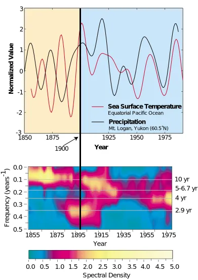
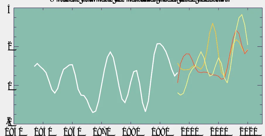
In the upper panel of figure 1 (page 13) two cli-matic timeseries are presented. One is the Niño 3.4 equato-rial Pacific sea surface temperature (SST) index as extended using proxy data (Kaplan et al., 1998). Note that the exten-sion of the SST index back in time is based on proxy data from remote sites which are highly correlated with SST in

the modern instrumental record. The validity of the ex-tended SST record thus rests, to some degree, on the as-sumption that this correlation was not different in the ear-lier period. The second curve is a record of precipitation derived from an ice core taken from Mt. Logan in the Yu-kon, Canada, at approximately 60.5˚N (Moore et al., 2001). Both timeseries have been low pass filtered with a cut-off period of 15 years to show decadal scale variability and normalized by subtracting the mean and dividing by the standard deviation.

Concentrate first on the more recent, blue, section of the panel. During this period, from 1900 to the present, the two records show a strong positive correlation, statisti-cally significant at the 99% level. This provides statistical evidence for an ENSO teleconnection influencing precipi-tation at this location. As is customary, the dynamical rea-son for this teleconnection is not fully understood, although it is clearly related to changes in the synoptic scale flow regime as seen in cross-correlation analysis of the Mount Logan timeseries with the annual 200 hPa geopotential field from the NCEP reanalysis 1948-1985, as shown in figure 2 (page 14) (Moore et al., 2001). Given the strong statistical correlation between these two records, and even some in-dication of the underlying causality, it would be fairly standard practice to, for example, extend the SST record back in time using the ice core data. Interestingly, in the older, yellow, portion of the panel the records are strongly anti-correlated, again at the 99% confidence level. Thus, our theoretical paleoreconstruction of SST based on this ice core data would produce variability of the incorrect sign. Climate predictions based on teleconnection patterns face exactly the same problem. A researcher with access to SST predictions in 1900, might confidently predict, based on the strength of correlation over the past 50 years, that pre-cipitation at Mt. Logan would continue to be anticorrelated. Again, the prediction would be of the wrong sign.

It is unclear what caused the change in the sign of the ENSO-Mt.Logan teleconnection around 1900. The lower panel presents the opportunity to engage in tantalizing speculation. This panel shows, on the same timescale as that above, anevolutionary spectral SST analysis derived from an annually resolved coral from Maiana atoll in the equatorial Pacific (Urban et al., 2000). The analysis was per-formed on 40-year segments of data overlapped by four years, using multitaper methods with red noise background assumptions. Around 1900, indicated by the vertical black line, was a period of time when the variability expressed in the coral record was shifting from primarily decadal to power to higher frequencies. This shift appears to corre-late with a shift in the phase of the correlation between the low frequency equatorial and extra-tropical response at Mt. Logan. Interestingly, tree-ring chronologies from high lati-tude sites in Alaska and Patagonia show a similar shift in coherence on the decadal time-scale around the same time (Villaba et al., 2001).

Leaving aside this rampant speculation, what can we conclude about decadal variability and climate predic-tion? Basically, the conclusion that this little story leads to is that understanding decadal variability of climate modes is difficult. Finding statistical significance in changes in interannual to decadal scale climate modes absolutely re-quires proxy based paleorecords that extend timeseries from the instrumental period. However, it is clear that no single proxy is sufficient. It is only with a wide geographi-cal range of accurately dated, independent proxies includ-ing documentary evidence, tree rinclud-ings, varved lake sediments, corals and ice cores that an understanding of decadal variability in climate teleconnections such as those associated with ENSO might evolve. And only then, will regional climate predictions based on these climate modes reliably transcend the assumption of statistical stationarity. Achieving such a thorough description and understand-ing of interannual to decadal climate variability is one of the primary goals of the CLIVAR/PAGES Intersection pro-gram. Interested readers are encouraged to become in-volved and to visit the CLIVAR (http://www.clivar.org) and PAGES (http://www.pages-igbp.org) websites for more information.

D.M. Sonechkin, N.N. Ivachtchenko

Hydrometeorological Research Center of Russia Moscow, Russia

[email protected]

After the seminal researches of Ed Lorenz the idea of the chaotic nature, i.e. instability and unpredictability, of the atmospheric variations of all scales won almost all of meteorologists. On the one hand, the practice of the present-day medium- and long-range weather forecasting corroborates this idea. Moreover, the power spectra of the higher-frequency atmospheric variations within the direct enstrophy and inverse energetic cascades (over the peri-ods from one day up to one-two months) look to be con-tinuous and without any sharp peaks. Such shape of the power spectra is an inherent property of the truly chaotic dynamics. On the other hand, the computations of the lower-frequency parts of the atmospheric spectra (over the periods more than one-two months) invariable reveal nu-merous peaks and bands of increased power energy (in addition to the trivial peaks of the annual period and its super harmonics) on a red-noise background. Of course, these peaks and bands are usually tested as statistically insignificant. But their observation in a huge number of atmospheric spectra is a proxy proof of their reality. The quasi-biennial oscillation (QBO) is the most often observed peak among these. First of all, QBO is clearly established in the temporal variations of the zonal winds within the equatorial lower stratosphere. But, the phenomenon is also observed in the variations of different atmospheric vari-ables within extratropics. A quite satisfactory explanation what is the direct driver of the QBO of the equatorial winds

was given by Lindzen and Holton (1968). But the general nature of QBO as a widespread phenomenon is unknown up to now.

In order to clear up the nature of QBO and other mentioned peaks and bands of increased power energy the notion of the so-called strange NONCHAOTIC attractor seems to be important. This notion was recently introduced by mathematicians to depict some aperiodic variations in the nonlinear dynamical systems forced by two or more periodic external forces at incommensurable frequencies. The variations excited by such a manner were found to be of the neutral stability, i.e. they are predictable without any limit even if their shapes are very complex. The phenom-enon of the strange nonchaotic attractor turned out to be most evident if the ratios of the forcing frequencies ones to others are “worst” irrational numbers such as the root X*_{=1.8393…of the cubic equation X}3_-X2_{-X-1=0. The power}

spectra of the strange nonchaotic variations consist of in-numerable power-energy peaks with very different magnitudes. It was proven that the re-distribution of the peaks on the frequency axis forms a self-similar structure, i.e. a zoom of any part of a spectrum being considered re-veals the peak re-distribution of the same character. But, in practical calculations, these spectra look like continuous ones, and their peaks seem to be statistically insignificant under the traditional tests. It is just the same that one can see in the lower-frequency atmospheric spectra.

Actually, the phenomenon of the strange nonchaotic attractor is well known in meteorology. An ex-ample is the oceanic and atmospheric tides. The tides are

References:

Kaplan, A., Cane, M., Y. Kushnir, A. Clement, M. Blumenthal, B. Rajagopalan, 1998: Analyses of global sea surface tempera-ture 1856-1991. J. Geophys. Res., 103, 18,567-18,589. Moore, G. W. K., G. Holdsworth, and K. Alverson, 2001:

Extra-tropical response to ENSO 1736-1985 as expressed in an ice core from the Saint Elias Mountain Range in north-western North America, Geophys. Res. Lett., submitted. Urban, F. E., J. E. Cole, and J. T. Overpeck, 2000: Influence of mean

climate change on climate variability from a 155-year tropi-cal Pacific coral record. Nature, 407, 989-993.

Villaba, R., R.D. D'Arrigo, E.R. Cook, G.C. Jacoby, G. Wiles, 2001: Decadal-scale climatic variability along the extra-tropical western coast of the Americas: Evidence from tree-ring records. In: Interhemispheric Climate Linkages. Ed.: V. Markgraf, Academic Press, 155-172.

excited by the gravitation interactions between Earth, Sun, and Moon. These interactions are quasi-periodic, and the tides are known to be of neutral stability. But, our aim here is to indicate that the notion of the strange nonchaotic attractor may be also used to model and predict the interannual and interdecadal atmospheric variations.

Mention in this context the so-called Chandler wobble in the Earth’s pole motion. The mean period of this wobble is about 14 months (1.2 year), and the ratio of its frequency to the frequency of the annual period seems to be similar to the “worst” irrational number Y=0.8393… derived from the above root of the cubic equation (Sidorenkov and Sonechkin, 1999). It is well known that the Chandler wobble excites a pole tide in the atmosphere. For certain, this pole tide forces the equatorial gravity and Kelvin waves that are known in the Lindzen – Holton theory to be the direct drivers of the QBO of the lower-stratospheric equatorial zonal winds. Although the mag-nitude of this pole tide is very small a nonlinear mecha-nism of its force enhancing like the so-called parametric resonance may be supposed. Some similar enhanced ef-fects of the pole tide may also be supposed for the atmos-pheric variations within extratropics.

Thus the atmosphere turns out to be forced by a quasi-periodic manner. Therefore, the power spectra of the atmospheric variations must reveal some, possible subtle, peaks at both annual and Chandlerian frequencies and their combinational harmonics. In particular, a sequence of some peaks must exist at the difference frequency Z=1-Y =0.1607… (the oscillation of the about 6.5 years period), Z2

(the oscillation of the about 40 year period) etc. as a conse-quence of the above-mentioned self-similarity of the power spectra of the strange nonchaotic attractor. This sequence can be also shifted along the frequency axis as a whole, so that all of the underlain periods are doubled, tripled, or quadrupled. For example, it is well known that the spec-trum of the equatorial QBO reveals the main peak at the frequency of the doubled Chandlerian period (of the about 28 months, i.e. 2.4 years). The doubled period correspond-ing to Z (of the about 13-14 years) is also observed (Vlasova et al. 1987). Unfortunately, the length of the equatorial lower-stratospheric zonal wind record is too short to ad-mit an accurate estimation of the energy of the wind oscil-lations at the frequency Z2_.

The ENSO spectra computed on the base of some essentially longer records reveal this peak clearly (Sonechkin and Wu Hongbao, 1999). It is interesting to mention that the ENSO records but the only ENSO spectra reveal a kind of self-similarity (Sonechkin et al. 1999). The well known maximal negative anomalies of the Southern Oscillation index near 1900s, 1941-42 and 1982-1983 coin-ciding with the greatest El Niños of the 20th century form the boundaries of the main constituents (of the about 40 year length) that form a self-similar structure of the tem-poral ENSO variations. Each of the constituents may be decomposed onto several parts the shapes of which turn out to be of the same character that is inherent to the main

constituents. Moreover, the same self-similar structure is seen in the temporal variations of the hemispheric mean surface air temperatures and the European temperatures as well (Sonechkin et al., 1999). The 65-70 year long tem-perature oscillation recognized by Schlesinger and Ramankutty (1994) reveals itself as an envelope of the above main constituents. In other words, this oscillation is a re-sult of the 40 years period doubling.

According to our estimation the contribution of all peaks considered and their innumerable harmonics into the general energy of the interannual and interdecadal at-mospheric variations is about 25% of the general energy. Even if the rest of the energy is a product of some truly chaotic processes connected with slowly varying compo-nents of the global climate system we believe that a new approach to the prediction of these variations may be de-veloped. The essence of this approach consists of the tak-ing into consideration the depicted strange nonchaotic char-acter of the quasi-periodic forced components of these. A certain robustness to the random distortions of the initial atmospheric data must be a prominent property of such prediction.

References

Lindzen, R.S., Holton, J.R., 1968: A theory of the quasi-biennial oscillation. J. Atmos. Sci., 25, 1095-1107.

Schlesinger, M.E., Ramankutty, N. 1994: An oscillation in the glo-bal climate system of period 65-70 years. Nature, 367, 723-726.

Sidorenkov, N.S., Sonechkin, D.M. 1999: Motions of the Earth’s pole as a dynamical three-frequency system. Astronomy Reports, 43, 556-560. Translated into English from Astronomicheskii Zhurnal, 1999, 76, 636-640.

Sonechkin, D.M., Astafyeva, N.M., Datsenko, N.M., Ivachtchenko, N.N., Jakubiak, B. 1999: Multiscale oscillations of the glo-bal climate system as revealed by wavelet transform of observational data time series. Theor. Appl. Climatol., 64, 131-142.

Sonechkin, D.M., Wu Hongbao 1999: Multiscale interrelations between air temperature in Southeast China and El Niño: wavelet analysis. Izvestiya, Atmospheric Oceanic Physics, 35, 227-235. Translated into English from Izvestiya A.N. Fizika Atmosfery i Okeana, 1999, 35, 250-258.

Midlatitude Ocean-Atmosphere Interaction in an idealized Coupled Model

S. Kravtsov, A. W. Robertson and M. Ghil Univ. of California, Los Angeles,

Dept. of Atmos. Sci., 405 Hilgard Ave., Los Angeles, USA [email protected]

1. Introduction

The midlatitude circulation in the upper ocean is forced by the atmospheric wind stress and advects sea surface temperature (SST) in the mixed layer, which, in addition, exchanges heat with the atmosphere. The heat flux anoma-lies due to SST changes may in turn affect the atmospheric flow. The objective of this study is to identify possible re-gimes of interannual-to-interdecadal timescale air-sea in-teraction in an idealized, nonlinear, quasigeostrophic ocean-atmosphere model that resolves baroclinic eddies in both the atmosphere and the ocean.

2. Model

The model (Dewar, 2000) consists of a single North Atlan-tic-size oceanic basin and a 2 x 104 _{km-long atmospheric}

channel. The coupling between the two-layer oceanic and atmospheric dynamical components occurs through a sim-ple mixed layer parameterization. The SST is advected by the currents in the mixed layer and affects the atmospheric circulations through the associated air-sea heat fluxes.

3. Main conclusion

We find that the atmospheric behaviour on timescales longer than interannual depends little on oceanic

dynam-ics. The dominance of the low frequencies in the power spectrum of the barotropic atmospheric field is shown to be due to internal atmospheric nonlinearities (cf. James and James, 1989). On the other hand, the oceanic low-frequency variability is primarily determined by the structure and time-dependence of the intrinsic atmospheric variability (cf. Saravanan et al., 2000).

4. Results

4.1 Model climatology

The atmospheric climatology is represented by a zonally-modulated climatological jet having a realistic amplitude. The relative locations of the jet maximum, storm track and maximum low-frequency barotropic activity are also real-istic. The time mean oceanic circulation consists of subtropi-cal and sub-polar gyres, which are separated by a midlatitude region of weak zonal current. This double midlatitude jet structure is similar to the Gulf Stream - Lab-rador current system.

4.2 Low-frequency variability in the model Leading mode of variability

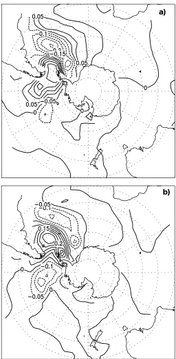
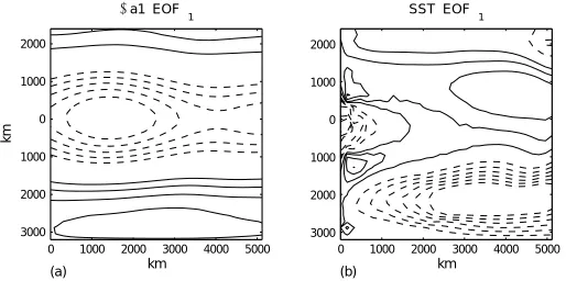
The leading pattern of atmospheric low frequency variabil-ity in the model involves intermittent equivalent barotropic highs and lows over the ocean (Fig. 1a). Associated with the low pressure anomalous atmospheric conditions is an SST anomaly, having positive values over most of the midlatitude and northern North Atlantic, with the excep-tion of the region in between the model Gulf Stream and Labrador currents, where negative values are seen (Fig. 1b).

Figure 1: Leading EOFs of (a) lower atmospheric layer streamfunction (41% of variance), CI 0.5 x106_m2_s-1_{; (b) sea surface}

tempera-ture (25% of variance), CI 0.1o_{C. Negative contours dashed, zero contours not plotted. The correlation between the corresponding 5}

yr low pass-filtered PCs is about 0.7.

0 1000 2000 3000 4000 5000

3000 2000 1000 0 1000 2000

km

km

Ψ

a1 EOF

1

(a)

0 1000 2000 3000 4000 5000

3000 2000 1000 0 1000 2000

SST EOF

1

Negative SST anomalies also occur in the tropical ocean, but these are not expected to be realistic. This air-sea pat-tern is similar to that observed by Kushnir (1994) in his analysis of interdecadal climate behavior in the North At-lantic. This SST distribution is accompanied by intensified model Gulf Stream and weakened model Labrador cur-rent. A spatial structure of the SST anomaly shows that it cannot be locally forced by anomalous air-sea fluxes.

Causes of variability

We have shown that in our model the SST pattern described above is directly forced by the atmospheric time-dependent wind, whose structure is not sensitive to, and is independent of, the oceanic evolution. In the western part of the ocean the SST response is largely due to the advection of mean SST by anomalous baroclinic currents associated with the wind anomaly. In the east, heat fluxes associated with the anomalous Ekman currents and en-trainment in the mixed layer dominate. There is a weak modulation of the SST structure by the heat flux, due to atmospheric temperature anomaly that accompanies the wind pattern.

Therefore, we propose an explanation of the long-term SST variability in the North Atlantic, which does not involve ocean-atmosphere feedbacks at all, nor the exist-ence of self-sustained or damped oceanic eigenmodes. In-stead, the atmospheric low-frequency pattern, which is in-ternally generated by atmospheric nonlinearities and has a specific spatial structure, directly causes changes in the oceanic circulation, which determine the SST response.

R.J. Haarsma and F.M. Selten

Royal Netherlands Meteorological Institute P.O. Box 201, 3730 AE De Bilt, The Netherlands [email protected]; [email protected]

One of the fundamental questions in current research about the mechanisms of decadal variability in the extra-tropics is the interplay between the ocean and the phere. Is the coupling between the ocean and the atmos-phere crucial for the generation of decadal variability and if so what is the nature of this coupling? We have tried to answer this question within the context of a climate model of intermediate complexity ‘ECBilt’, developed in the pre-dictability division of the Royal Netherlands Meteorologi-cal Institute (KNMI).

ECBilt was developed with the purpose of simulat-ing qualitatively correctly the extra-tropical climate, with special focus on the simulation of the position and strength of the storm tracks and dominant modes of variability. The dynamical core of ECBilt is a quasi-geostrophic T21 model with 3 vertical levels. The diabatic processes are modelled using simple parameterisations. A full hydrological cycle is included. ECBilt is coupled to a coarse primitive

equa-tion ocean model with a horizontal resoluequa-tion of 5.6 de-grees and 12 vertical levels. Sea-ice growth is simulated with a zero layer thermodynamic model. A detailed de-scription of ECBilt and its performance can be found in Opsteegh et al. (1998). The main advantage of ECBilt is that due to its relative simplicity and low computational cost carefully additional simulations can be performed to un-ravel cause and effect relationships of the phenomena simu-lated in ECBilt.

We have investigated decadal variability in the North Atlantic and in the Southern Ocean as examples of extra-tropical decadal variability.

North Atlantic

There is observational evidence for typical sea surface tem-perature (SST) variations in the North Atlantic on a time scale of 10 to 15 years (Deser and Blackmon, 1993). At the same time, a typical sea level pressure (SLP) variation is observed in the atmosphere, which resembles the North Atlantic Oscillation (NAO). A singular value decomposi-tion (SVD) analysis of SST and 800 hPa geopotential height in a thousand year control integration of ECBilt, revealed a mode (Fig.1, page 9) with a dominant time scale of 16-18

Importance of the meridional position of the atmospheric variability

All the basin scale oceanic responses described above cru-cially depend on the meridional position of the atmospheric activity centre relative to the oceanic gyres. If the two posi-tions are not in mutual adjustment, as they are in the cou-pled run, the details of the basin scale SST modes are al-tered. This occurs through changes in the relative ampli-tudes and spatial structure of different feedbacks in the mixed layer evolution. Thus, the spatial structure of atmos-pheric variability is crucial in determining the oceanic time dependence in the model.

References

Dewar, W. K., 2000: Quasigeostrophic climate dynamics. J. Mar. Res, submitted.

James, I. N., and P. M. James, 1989: Ultra-low frequency variabil-ity in a simple atmospheric circulation model. Nature, 342, 53-55.

Kushnir, Y., 1994: Interdecadal variations in North Atlantic sea surface temperature and associated atmospheric condi-tions. J. Climate, 7, 141-157.

Saravanan, R., G. Danabasoglu, S. C. Doney, and J. C. McWilliams, 2000: Decadal variability and predictability in midlatitude ocean- atmosphere system. J. Climate, 13, 1073-1097.

yr in SST (Selten et al., 1999). This mode is similar to the first canonical correlation analysis (CCA) mode found by Grötzner et al. (1998) from observed SST and SLP. This ob-served mode peaks around a somewhat shorter time scale of about 12 yr. The 16-18 yr mode in SST in ECBILT is re-lated to an oceanic subsurface oscillation which shows a clockwise propagation in the subtropical gyre (Fig.2, page 8). Additional experiments have revealed much of the un-derlying mechanism. In order to investigate the role of oce-anic forcing on the atmospheric circulation for the decadal mode we performed the following experiment: We repeated the 1000-yr coupled integration but on an arbitrary year we decoupled the atmosphere from the ocean. From that year onward we used the daily SST values and sea-ice cover

of that year as the lower boundary condition for the at-mosphere. The ocean and the sea-ice are forced by the vary-ing atmosphere. Thus the ocean is forced with fluxes that depend on the actual SST values, whereas the surface heat fluxes that the atmosphere receives depend on the pre-scribed SST. We will denoted this experiment as one-sided coupling. The SVD patterns of this one-sided coupled run are virtually the same as the SVD patterns of the coupled run. The spectra of the time series of these patterns are changed: They are less red and the dominant peak at 16-18 yr in SST has disappeared. In the subsurface of the ocean the oscillation with a time scale of 16-18 yr is however still present although significantly weaker. This demonstrates that the time scale of the 16-18 yr mode is set in the ocean

b) a)

Figure 1: Covarying anomaly patterns of wintermean SST (a) and 800 hPa geopotential height (b). The amplitude variations of both are well correlated (0.7), with the atmospheric circulation anomaly forcing the SST anomaly.

and that a dynamic coupling between the ocean and the atmosphere is not necessary for the generation of this time scale. The less red spectrum and the disappearance of the peak in the SST are due the fact that in the one-sided cou-pling experiment the atmosphere is seen by the ocean as having an infinite heat capacity, because the overlying sur-face air temperature (SAT) does not adjust to the SST’s, re-sulting in abnormally large surface fluxes and a rapid damping of the generated SST anomalies. The adjustment of SAT to the SST is thus crucial for the subsurface decadal time scale to be manifest at the surface. Additional sensi-tivity experiments have revealed that the dominant proc-ess for the generation of the 16-18 yr time scale are varia-tions in the ocean salinity field. The subsurface tempera-ture mode is accompanied by variations in the surface sa-linity. These salinity variations are responsible for the phase reversal in the subsurface mode by affecting convection off the coast of New Foundland. An additional experiment in which the windstress was prescribed revealed that the feedback of wind anomalies on the ocean gyre circulation is not essential for the generation of 16-18 yr mode. The windstress feedback enhances the amplitude of this mode through anomalous Ekman pumping, which is responsi-ble for a deeper mixing of SST anomalies, resulting in sub-surface anomalies with a larger thermal inertia.

Southern Ocean

In the same thousand year simulation of ECBilt, propagat-ing SST variations are found in the Southern Oceans around the Antarctic continent at a typical timescale of 8 years. (Haarsma et al., 2000). These variations resemble the so-called Antarctic Circumpolar Wave (White and Peterson, 1996), characterized by alternating warm and cold SST anomalies propagating around the Antarctic continent in about 8 years. Additional experiments have shown that the mechanism for this 8 yr mode around Antarctica is very similar to mechanism for the 16-18 yr mode in the North Atlantic: The SST anomalies are generated by anomalies in the atmospheric circulation and are accompanied by a sub-surface oscillation in the ocean, which propagates eastward around Antarctica (Fig. 3). The main difference is in the ocean dynamics setting the time scale. For the 8 yr mode around Antarctica the advective resonance mechanism of Saravanan and Mc Williams (1998), appears to be respon-sible for the dominant time scale. In the advective reso-nance mechanism the preferred time scale is set by the ra-tio of the horizontal scale of the dominant atmospheric forc-ing patterns and the advection velocity of the ocean cur-rents. An experiment in which we doubled artificially the strength of the Antarctic circumpolar current (ACC) re-vealed that the time scale of the mode was halved from 8 yr to 4 yr. An additional simulation with climatological salinity values in the ocean density calculations revealed that the effect of salinity anomalies, which were crucial for the North Atlantic mode, are of minor importance for this mode.

The simulations with ECBilt support the following picture of decadal climate variations over the oceans and surrounding continents: Atmospheric circulation

anoma-lies force typical patterns of SST anomaanoma-lies, which are mixed to deeper layers due to Ekman pumping, in response to anomalous windstress. The ocean response to these anomalies gives rise to a preferred timescale which is im-printed back on the atmosphere primarily on the surface air temperature. The response of the atmospheric circula-tion to the SST anomalies is weak an not crucial for the preferred time scale. The thermodynamic adjustment of SAT to the SST anomalies enhances the persistence of SST anomalies and makes the subsurface signal manifest at the surface. In the North Atlantic salinity anomalies are essen-tial for the generation of the preferred time scale, whereas in the Southern Ocean this time scale is set by the

advec-b) a)

tive resonance mechanism of Saravanan and McWilliams.

References:

Deser, C., and M.L. Blackmon, 1993: Surface climate variations over the North Atlantic Ocean during winter 1900-1989. J. Climate, 6, 1743-1753.

Grötzner, A., M. Latif, and T.P. Barnett, 1998: A decadal climate cycle in the North Atlantic ocean as simulated by the ECHO coupled GCM. J. Climate, 11, 831-847.

Haarsma, R.J., F.M. Selten, and J.D. Opsteegh, 2000: On the mecha-nism of the Antarctic Circumpolar Wave. J. Climate, 13, 1461-1480.

Rowan Sutton

Centre for Global Atmospheric Modelling University of Reading, Reading, UK [email protected]

Understanding fluctuations of the climate system on time scales from decades to centuries is one of the major topics of the CLIVAR programme. Five Principal Research Areas (PRAs) within the Initial CLIVAR Implementation Plan (WCRP, 1998) focus on aspects of decadal climate variabil-ity. In the Atlantic Sector the key topics are the North At-lantic Oscillation, the Thermohaline Circulation and Tropi-cal Atlantic Variability. The problem of understanding and forecasting these aspects of decadal climate variability presents a major challenge to the scientific community. An adequate response is beyond the resources of any single organisation, and thus coordination of activities is essen-tial. PREDICATE is a 3-year research programme, funded by the European Union under Framework 5, in which eight of the leading climate centres in Europe have come together to provide a focused effort in this vital area.

The objectives of PREDICATE are:

1. To assess the predictability of decadal fluctuations in Atlantic-European climate.

2. To improve understanding and simulation of mechanisms via which ocean-atmosphere interac-tions cause decadal fluctuainterac-tions in Atlantic-Euro-pean climate.

3. To improve the European capability for forecast-ing decadal fluctuations in Atlantic- European cli-mate by developing forecasting systems based on coupled ocean-atmosphere models.

4. To work with targeted user groups to assess the potential benefits from possible future decadal fore-casts for selected sensitive industries.

As can be seen, PREDICATE targets the role of ocean-atmosphere interactions rather than the response to exter-nal forcings. These aims are to be achieved through a coor-dinated programme of numerical experimentation,

evalu-ation against observevalu-ations, and development of prediction systems. The project has four principal themes, as follows.

A) Mechanisms and Predictability of Decadal Fluctua-tions in the Atmosphere.

The potential predictability of the North Atlantic Os-cillation (NAO) has been a subject of considerable recent debate. It has been shown that atmosphere models forced with observed SST can simulate NAO variability that is highly correlated with the observed record (Rodwell et al., 1999). Because of large sampling fluctuations there is need for caution in the interpretation of these results (Mehta et

PREDICATE: Mechanisms and Predictability of Decadal Fluctuations in Atlantic-European Climate

Opsteegh, J.D., R.J. Haarsma, and F.M. Selten, 1998: ECBILT: A dynamic alternative to mixed boundary conditions in ocean models. Tellus, 50A, 348-367.

Saravanan, R., and J.C. McWilliams, 1998: Advective ocean-at-mosphere interaction: An analytical stochastic model with implications for decadal variability. J. Climate, 11, 165-188. Selten, F.M., R.J. Haarsma, and J.D. Opsteegh, 1999: On the mecha-nism of North Atlantic decadal variability. J. Climate, 12, 1956-1973.

al., 1999, Bretherton and Battisti, 2000), but they have yet to be fully explained. In some models there appears to be no significant skill (L. Terray, personal communication), and in those where skill exists it is not clear whether consistent features of the SST variability are responsible.

A major contribution of PREDICATE to this topic is a rigorous quantitative comparison of four different atmos-phere GCMs to assess their skill in simulating the climate variability that was observed over the last century, with a particular focus on the North Atlantic region. The compari-son includes the powerful technique of signal-to-noise optimised Principal Component Analysis (Venzke et al., 1999). This approach enables determination of which fea-tures in the SST field exert most influence.

B) Mechanisms of Decadal Fluctuations in the Atlantic Ocean

Prominent amongst the observational results of re-cent years has been the identification of persistent, often propagating, surface and subsurface anomalies in the North Atlantic ocean (e.g. Dickson et al., 1988; Sutton and Allen, 1997; Curry and McCartney, 1998). A major current chal-lenge is to understand the mechanisms through which these anomalies form, propagate, and decay, and to understand how their life-cycles are related to fluctuations in the at-mosphere and in the oceanic gyre and thermohaline circu-lations.

In PREDICATE these issues are being addressed through a coordinated programme of experimentation with six different ocean GCMs. PREDICATE partners are inves-tigating the skill with which the variability observed in the Atlantic during the second half of the twentieth century is simulated in models forced with observed winds and air-sea fluxes. The sensitivity of simulations to model resolu-tion and the representaresolu-tion of the Arctic ocean is being ex-plored.

C) Decadal Climate Prediction for the Atlantic European Region.

The problem of decadal climate forecasting presents considerable scientific and technical challenges. Predictabil-ity on these timescales arises from two influences: that of the ocean, and that of external forcings such as the rising trend of greenhouse gases. Current climate change fore-casts make no use of information about the present state of the oceans (see Figure, page 1). This approach is very un-likely to be optimal for forecasts with time horizons of a few years or decades. Thus work to incorporate ocean state information into climate forecasts is essential.

Building on the understanding and evaluation of mechanisms achieved in other parts of the programme, a major part of PREDICATE is addressing the development of systems for decadal forecasting and the assessment of predictability on decadal timescales. The study of Griffies and Bryan (1997) was a pioneering step in this field. How-ever, the coarse resolution of the model used brings into

question the realism of the mechanisms it simulated. PREDICATE will take forward the work of Griffies and Bryan by performing experimental decadal predictions with four different coupled models, all of which have higher resolution than that used by Griffies and Bryan. The sensitivity of forecasts to initial conditions in both the ocean and the atmosphere will be investigated and a quan-titative assessment of decadal predictability will be made for each of the models. The application to decadal fore-casting of techniques (e.g. ‘breeding’) to generate initial perturbations for decadal forecasts will be investigated.

D) Interactions with Users and Dissemination of Results.

Decadal time horizons are of central concern for stra-tegic planning in a wide range of industries. It is a high priority for PREDICATE that the needs of potential users are well understood and are taken into account through-out the programme. It is also essential that potential users begin to think seriously about how they could exploit fu-ture real-time decadal forecasts. To achieve these ends PREDICATE is promoting a dialogue between the climate prediction science community and business users in a wide range of sectors (for example, insurance, energy, water, con-struction). An example of the project activities is a work-shop at The Royal Society London, 8-9 March 2002: ‘Cli-mate Risks to 2020: Business Needs and Scientific Capa-bilities’

The PREDICATE project began on 1 March 2000 and will end on 28 February 2003. The PREDICATE partners are:

CGAM: Centre for Global Atmospheric Modelling, Uni-versity of Reading, UK, The Met Office, Bracknell, UK, MPI: Max Planck Institut für Meteorologie, Hamburg, Ger-many, LODYC: Laboratoire d’Oceanographie Dynamique et de Climatologie, Paris, France, NRSC: Nansen Environ-mental and Remote Sensing Research Centre, Bergen, Nor-way, ING: Istituto Nazionale di Geofisica, Bologna, Italy., DMI: Danmarks Meteorologiske Institut, Copenhagen, Denmark, CERFACS: The European Centre for Research and Advanced Training in Scientific Computation, Tou-louse, France.

For further information see http:// ugamp.nerc.ac.uk/predicate

References:

Bretherton, C.S., and D.S. Battisti, 2000: An interpretation of the results from atmospheric general circulation models forced by the time history of the observed sea surface tem-perature distribution. Geophys. Res. Lett., 27, 767-770. Curry, R.G., and M. S. McCartney, 1998: Oceanic transport of

subpolar climate signals to mid-depth subtropical waters. Nature, 391, 575-577.

Dickson, R. R., J. Meincke, S.-A. Malmberg, and A. J. Lee, 1988: The Great Salinity Anomaly in the northern North Atlan-tic 1968-1982. Prog. Oceanogr., 20, 103-151.

Griffies, S.M., and K. Bryan, 1997: A predictability study of simu-lated North Atlantic multidecadal variability. Climate Dy-namics, 13, 459-487.

Alverson et al., page 4: Improving Climate Predictability and understanding Decadal Variability using Proxy Climate Data

Year

0.0 0.5

1.0 1.5 2.0

2.5 3.0

3.5 4.0 4.5 5.0

Spectral Density

1855

1875

1895

1915

1935

1955

1975

Frequency (years

-1

) 0.0

0.1

0.2

0.3

0.4

0.5

10 yr

5-6.7 yr

4 yr

2.9 yr

-3

-2

-1

0

1

2

3

1850

1900

1950

1975

1875

1925

Sea Surface Temperature

Equatorial Pacific Ocean

Precipitation

Mt. Logan, Yukon (60.5˚N)

Normalized Value

Year

Figure 2: Cross-correlation of the Mount Logan annual snow accumulation timeseries with the annual 200 mb geopotential field from the NCEP reanalysis 1948-1985. The field is displayed at those points where the cross-correlation is sig-nificant at the 95% level. The location of Mount Logan is indicated by the ‘*’. The Niño 3.4 region is bounded by the blue box.

Alverson et al., page 4: Improving Climate Predictability and understanding Decadal Variability using Proxy Climate Data

*

80oE 120oE 160oE 160oW 120oW 80oW

40oS 20oS 0o 20oN 40oN 60oN 80oN

-0.6 -0.3 0 0.3 0.6

10 25 50 75

Eleven model ensemble percentage of "potential predictability" for decadal means

Boer, page 3: Decadal potential predictability in coupled models

Mehta, V.M., M.J. Suarez, J. Manganello, and T.L. Delworth., 2000: Oceanic influence on the north atlantic oscillation and as-sociated northern hemisphere climate variations. Geophys. Res. Lett., 27, 121-124.

Rodwell, M.J., D.P. Rowell, and C.K. Folland, 1999: Oceanic forc-ing of the winter North Atlantic Oscillation and European Climate. Nature, 398, 320-323.

Arnaud Czaja and John Marshall Department of Earth, Atmospheric and Planetary Sciences

Massachussets Institute of Technology Cambridge, MA 02139, USA

[email protected]

1. Introduction

To explore evidence and possible mechanisms of decadal variability and atmosphere-ocean coupling, we introduce and study a simple SST index, ∆T; from a long observa-tional record (1856 - 1998); it measures the strength of the dipole of SST that straddles the Gulf Stream and was cho-sen because (i) it is a measure of low level baroclinicity to which cyclogenesis at the beginning of the Atlantic storm-track may be sensitive (ii) it may contain a signature of anomalies in ocean heat transport associated with both wind driven gyres and thermohaline circulation. We show that pronounced decadal signals in ∆T are found which covary with the strength of sea level pressure (hereafter SLP) anomalies over the Greenland - Iceland Low and sub-tropical High regions. Using the simple coupled model developed in Marshall et al. (2000), we interpret features of the power spectrum of observed SST and SLP as the sig-nature of coupled interactions between the atmospheric circulation and an anomalous wind driven ocean gyre and thermohaline circulation.

A much fuller discussion of the observational study summarized here, which builds on that of Deser and Blackmon (1993) - see also Grötzner et al. (1998) for a rel-evant modelling study - can be found in Czaja and Marshall (2001).

2. A cross Gulf Stream SST index

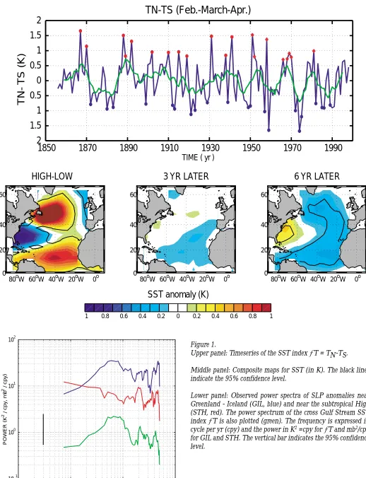
Figure 1 (upper panel) shows the time evolution of the SST index ∆T = TN-TS (difference of SST averaged over

[60˚-40˚W; 40˚-55˚N] and [80˚-60˚W; 25˚-35˚N] in late winter – February through April), from Kaplan et al. (1997)1. Typi-cal fluctuations of 1 K are found on interannual timesTypi-cales (blue curve), and represent fluctuations of 10 - 20 % of the

mean cross Gulf Stream SST gradient. As seen in Fig. 1 (page 16), they are reduced by about a factor of two on decadal timescales (green curve, 6- yr running mean). Using a com-posite analysis we investigate the typical evolution of the SST pattern captured by ∆T once it has been generated (Fig. 1, middle panel). Figure 1, middle panel, is obtained by compositing SST using high index years (red stars), using low index years (blue stars), and then subtracting low from high (to yield the High-Low plot); the same but using years shifted along by three relative to the stars (3 years later) and by six years (6 years later). High-Low reveals the tripole pattern (Fig. 1, middle panel, left plot) which evolves in time with damped oscillatory behaviour. No large scale signal is found three years after the tripole has been gener-ated (Fig. 1, middle panel, middle plot), but it reappears 6 yrs later with opposite sign (Fig. 1, middle panel, right plot). When the analysis is made using longer lags, there is a hint of reappearance of the initial tripole after 12-14 yrs, but the statistical significance is lost (not shown). Based on a simi-lar composite analysis with the long observational record of SLP by Kaplan et al. (1999), we find that atmospheric conditions which occur simultaneously with ∆T are remi-niscent of the North Atlantic Oscillation (NAO) signature in SLP (not shown), although shifted slightly southwest-ward. They show opposite-signed anomalies over the Greenland - Iceland Low (hereafter GIL) and subtropical High (hereafter STH) regions, such that in years when SST are warmer north than south of the Gulf stream (∆T > 0), the surface atmospheric circulation is weakened.

3. Spectral analysis

Figure 1 (lower panel) shows the observed power spectra for ∆T (green), GIL (blue) and STH (red). In agreement with the damped oscillatory behaviour displayed by the SST tripole (Fig. 1, left panel), but sharply contrasting with the traditional red noise prediction of Frankignoul and Hasselmann (1977), the power spectrum of ∆T shows a broad peak in the decadal band, with no attening on longer timescales. Rather, the power in the ∆T index continues to decrease with increasing timescale. The power spectra of GIL and STH are similar up to timescales of about 25 yrs (blue and red curves respectively in Fig. 1, lower panel). This is consistent with a spectral coherence analysis, which indicates strong coherence and a robust out of phase rela-tionship between GIL and STH up to 25 yrs (not shown), in agreement with the NAO paradigm. On longer

Sutton, R.T., and M. R. Allen, 1997: Decadal predictability of North Atlantic sea surface temperature and climate. Nature, 388, 563-567.

Venzke, S., M. R. Allen, R. T. Sutton, and D. P. Rowell, 1999: The atmospheric response over the North Atlantic to decadal changes in sea surface temperature. J. Climate, 12, 2562-2584.

Role of Ocean Dynamics and Atmosphere – Ocean coupling in the observed North Atlantic Decadal Variability

1

1850

1870

1890

1910

1930

1950

1970

1990

2

1.5

1

0.5

0

0.5

1

1.5

2

TIME ( yr )

TN-

TS (K)

TN-TS (Feb.-March-Apr.)

HIGH-LOW

80oW 60oW 40oW 20oW 0o

0 20 40 60

3 YR LATER

80oW 60oW 40oW 20oW 0o

0 20 40 60

6 YR LATER

80oW 60oW 40oW 20oW 0o

0 20 40 60

1 0.8 0.6 0.4 0.2 0 0.2 0.4 0.6 0.8 1

SST anomaly (K)

10 3 10 2 10 1 100

10 1 100 101 102

FREQUENCY (cycle per yr)

POWER (K

2 / cpy, mb 2 / cpy)

Figure 1.

Upper panel: Timeseries of the SST index ∆_{T = TN-TS.}

Middle panel: Composite maps for SST (in K). The black lines indicate the 95% confidence level.

Lower panel: Observed power spectra of SLP anomalies near Greenland - Iceland (GIL, blue) and near the subtropical High (STH, red). The power spectrum of the cross Gulf Stream SST index ∆T is also plotted (green). The frequency is expressed in cycle per yr (cpy) and the power in K2 _{=cpy for} ∆_{T and mb}2_/cpy

timescales, however, the two spectra have different struc-tures and the coherence between them is reduced (not shown). While the STH power spectrum keeps increasing with time scales, that of GIL decreases. The NAO index of Hurrell (1995), the normalized SLP difference between Ice-land and Lisbon, has a power spectrum very similar to that of STH (not shown).

4. Discussion

Perhaps the most striking feature of the analysis present here is the decrease of power seen in both ∆T and GIL spec-tra at timescales longer than about 25 yrs. The latter can be captured by a simple coupled stochastic model (Marshall et al., 2000), and, in that model, arises essentially because the ocean circulation is assumed to play a role in advecting heat from the warm lobe to the cold lobe of the dipole (i.e. down gradient), but with some delay. Much further work is needed to fully determine what ocean dynamics might be responsible for the delay, and the role of Atmosphere -Ocean coupling in the decadal variability displayed by the SST tripole and GIL presented here. Our observational re-sults suggest that a weak coupling is present through con-trol of the strength of GIL by ocean circulation at low - fre-quency, presumably through its impact on SST and sur-face baroclinicity measured by ∆T. As discussed in detail in Czaja and Marshall (2000), predictive skill in the 10 to 20 year band is nevertheless expected to be low, owing to the small quality factor of the coupled oscillation.

Alexander B. Polonsky

Marine Hydrophysical Institute., 2 Kapitanskaya St., 335 000 Sevastopol, the Crimea, Ukraine

[email protected]

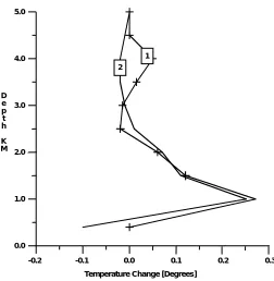
Ocean variability is most likely a crucial factor in regulating the interdecadal-to-multidecadal natural changes in the coupled ocean-atmosphere system and, hence, the low-frequency climate variability (Bjerknes, 1964; WCRP, 1998). At the same time, the Ocean damps the glo-bal warming through the changes of meridional heat trans-port and latent heat fluxes (Polonsky and Voskresenskaya, 1996; Voskresenskaya and Polonsky, 1994). So, the reliable detection of the low-frequency ocean variability is crucial factor to study the long-term (natural and human-induced) climate changes. Because of the limitations in the quantity and quality of oceanographic observations there is a prob-lem of detection of the climatic signals in deep-ocean lay-ers. The brief discussion of this problem is aim of present note with strong focus to the North subtropical Atlantic. More complete discussion will be published soon (Polonsky, 2001).

Deep-sea observations have been performed for more than a century. Before the 1970’s, Nansen profiles were the main source of deep-sea data. Then the XBT and CTD soundings essentially replaced the Nansen measurements.

However, the routine oceanographic observations are too sparse and noisy for the reliable detection of long-term changes of the oceanic fields in the deep ocean (below about upper 0.8-1 km layer). Even in the regions with the best coverage (such as North subtropical Atlantic), only small portion of the profiles reached the deep layers (especially before the WOCE programme) and observational activity was concentrated in recent decades (Fig. 1, page 18). This means that even there, only decadal-scale (not longer-term) variations in the upper (˜1km) layer may be estimated with

reasonable accuracy (signal-to-noise ratio ≥1). Regular XBT profiles have been collected during the recent 35 years and the maximum depth of XBT sounding is usually 800 m. In addition, there was an essential decrease of XBT activity after 1979. Therefore the XBT data cannot eliminate the lack of long-term deep-sea observations (see also, White, 1995). As a result there are at least two following problems: (a) the reliable detection of long-term variations of deep-ocean layers and (b) the separation of trend-like and low-fre-quency quasi-periodical signals. Unique observations per-mit different interpretations. I would like to demonstrate this point for the North Atlantic subtropical gyre using fol-lowing remarkable example.

Parrilla et al. (1994) found significant and quite uniform warming in deep Atlantic Ocean along 24˚N

be-References

Czaja A., and J. Marshall, 2000: On the interpretation of AGCMs response to prescribed time varying SST anomalies. Geophys. Res. Lett., 27, 1927-1930.

Czaja A., and J. Marshall, 2001: Observations of Atmosphere-Ocean coupling in the North Atlantic. Quart. J. Roy. Me-teor. Soc., submitted.

Deser C., and M. L. Blackmon, 1993: Surface climate variations over the North Atlantic Ocean during winter: 1900-1989. J. Climate, 6, 1743-1753.

Frankignoul, C., and K. Hasselmann, 1977: Stochastic climate models, part II: application to sea-surface temperature variability and thermocline variability. Tellus, 29, 289-305. Grötzner, A., M. Latif, and T.P. Barnett, 1998: A decadal climate cycle in the North Atlantic Ocean as simulated by the ECHO coupled GCM. J. Climate, 11, 831-847.

Hurrell, J., 1995: Decadal trends in the North Atlantic Oscillation: regional temperature and precipitation. Science, 269, 676-679.

Kaplan A., Y. Kushnir, M. Cane, and B. Blumenthal, 1997: Reduced space optimal analysis for historical datasets: 136 years of Atlantic sea surface temperatures. J. Geophys. Res., 102, 27,835-27,860.

Kaplan A., Y. Kushnir, and M. Cane, 2000: Reduced space opti-mal interpolation of historical marine sea level pressure: 1854-1992. J. Climate, 13, 2987-3002.

Marshall, J., H. Johnson, and J. Goodman, 2001: A study of the interaction of the North Atlantic Oscillation with the ocean circulation. J. Climate, in press.

tween 1957 and 1992. It was at a maximum (>0.25˚C) be-tween 1 and 2 km. “However, to what degree those ob-served changes represent large-scale volume changes or whether they occurred largely due to variations of the lo-cation of the gyre is not clear” (WCRP, 1998). Figure 2 shows that the latter assumption is very likely true. If subtropical gyre has shifted to the South by about 2˚ from 1957 to 1992 even without any other changes, it results in the deep-ocean temperature change along 24˚N resembling the warming

described by Parrilla et al. (1994). In fact the intensification of the subtropical gyre occurred also in that time. Figure 3 demonstrates that the multidecadal quasi-periodical rise of the sea level pressure (SLP) in the Azores High and as-sociated increasing of the Rossby (NAO) index from late 1950’s to early 1990’s have been accompanied by the dis-placement of the Azores High to the Southwest. This should be accompanied by the intensification and southward shift of the Subtropical gyre. Thus the warming observed by Parrilla et al. (1994) is likely the manifestation of multidecadal temperature variability due to changes of the location and intensity of the Atlantic Subtropical gyre as part of the coupled ocean-atmosphere system variability.

Certainly, it is next to impossible to distinguish the natural multidecadal changes and human-induced warm-ing of deep-ocean layers because the amount of available deep-ocean data is absolutely insufficient to separate the trend-like and low-frequency quasi-periodical signals in the extended ocean interior. Both of them look like long-term tendencies. Of course, the problem of separation of the human-induced warming and natural multidecadal changes is not so simple in principle even if one has the high-resolved long-term global observations (see e.g., dis-cussion of this problem from the atmospheric point of view in Nature [Corti et al., 1999 and Hasselmann, 1999]). It is clear however, without such observations this is impossi-ble at all. It concerns also the entire climate system includ-ing deep-ocean layers.

This should be noted, the long-term meteorologi-cal data provide some arguments for separation of the hu-man-induced and natural multidecadal changes. For in-stance, the multidecadal and longer-term tendencies of subtropical SLP are opposite one another because the cen-tury trend-like Azores High deepening is accompanied by its shift to the North (Fig.3). There are also the essential differences between decadal-scale and multidecadal modes (Enfield and Mestas-Nunez, 1999; Polonsky et al., 1997). This is a result of differences between mechanisms those are responsible for the century-scale, multidecadal and decadal-scale changes in the ocean-atmosphere-land sys-tem. First of them is due likely to the human-induced proc-esses, while the second and third ones are due mostly to the natural variability (changes of the global and basin-scale variability of the coupled system, respectively) (Polonsky, 2001). To clarify the relative importance of dif-ferent mechanisms and their possible interaction it is a stra-tegic task for the future. The ocean observational pro-gramme is an important element of this strategy.

Thus, what should we do during the next few dec-ades for the development the study of the long-term cli-matic variability of the coupled ocean-atmosphere system on the globe, taking into account an uncertainty of climate ocean change due to lack of deep-ocean observations? It is clearly necessary to perform precise global (including deep-ocean) observations. However, a fast progress in the study of the long-term variability of climatic system using instru-mental deep-ocean data is not likely. Duration of

observa-Temperature Change [Degrees]

-0.2 -0.1 0.0 0.1 0.2 0.3

5.0 4.0 3.0 2.0 1.0 0.0 D e p t h K M 1 2

Number of the NODC deep-sea observations over the globe

1 - XBT data

2 - CTD/STD data

3 - Nansen bottles N u m b e r o f O b s e r v a t i o n s 60,000 40,000 20,000 0

1940 1960 1980

Years

1

3

2

Fig. 2: Change of zonally averaged temperature in the North Atlantic Ocean as a function of depth: 1-difference of climate temperature at 25˚N and 23˚N calculated using NODC data; 2-observed by Parilla et al (1994) difference at 24˚N between 1992 and 1957.

tions should be at least of the same order as the typical time scale of processes to be studied. This means we should continue to support the global observational network at least during the next few decades and put attention to analysis of different kinds of observations. Precise long-term deep-ocean observations, such as WOCE soundings, are absolutely necessary for the study of low-frequency cli-matic change. Essential decreasing of the ocean observa-tional activity as happened in the beginning of the satellite era (see Fig.1A) is inadmissible. This manifested among the others in the cessation of international subsurface ob-servations at the Ocean Weather Stations. It is absolutely clear, the observations using new technology should con-tinue the long-term time series and should not lead to their interruption.

References

Bjerknes, J., 1964: Atlantic air-sea interaction. Advance in Geophys-ics, 10, 1-82.

Corti, S., F. Molteni, and T.N.Palmer, 1999: Signature of recent climate change in frequencies of natural atmospheric cir-culation regimes. Nature, 398, 799-802.

Enfield D., and A.M. Mestas-Nunez, 1999: Multiscale variability in global SST and their relationships with tropospheric cli-mate patterns. J. Clicli-mate, 12, 2719-2733.

Hasselmann K., 1999: Climate change: Linear and nonlinear sig-natures. Nature, 398, 755-756.

Hurrell, J.W., 1995: Decadal Trends in the North Atlantic Oscilla-tion: Regional Temperatures and Precipitation. Science, 269, 676-679.

Levitus, S., and R.D. Gelfeld, 1992: National Oceanographic Data Center inventory of physical oceanographic profiles. U.S. De-partment of Commerce, NOAA, Washington, D.C., USA, 242.

Levitus, S., and T.P. Boyer, 1994: NOAA Atlas NESDIS 4. Ibid, 117. Machel, H., A. Kapala, and H. Flohn, 1998. Behaviour of the cen-tres of Action Above the Atlantic since 1881. Part 1: Char-acteristics of seasonal and interannual variability. Int. J. Climatology, 18, 1-22.

Parrilla, G., A. Lavin, H.Bryden, M.Garcia, and R.Millard, 1994: Rising temperature in the subtropical North Atlantic Ocean over the past 35 year. Nature, 369, 48-51.

Polonsky, A., 2001: Is warming of intermediate waters of the North Atlantic subtropical gyre really observed. J. Phys. Ocea-nography, in press.

Polonsky, A.B., and E.N. Voskresenskaya. Low-frequency vari-ability of meridional drift transport in the North Atlantic. Russian Meteorology and Hydrology, No.7, 66-74, 1996, (Translated from Russian and Published by Allerton Press in the USA).

Polonsky, A., E. Voskresenskaya, and V. Belokopytov, 1997:. Vari-ability of northwestern Black sea hydrography and river discharges as part of global ocean-atmosphere fluctuations. In: Sensitivity to Change: Black Sea, Baltic Sea, North.Sea. Kluwer Academic Publishers, 11-24.

Voskresenskaya, E.N. and A.B. Polonsky, 1994: Low-frequency variability of heat fluxes in the North Atlantic. Russian Me-teorology and Hydrology, 9, 37-44.

WCRP, 1998: CLIVAR Initial Implementation Plan. WCRP WMO/ TD No. 869, ICPO, No. 14, 314pp.

White W.B., 1995: Design of a global Observation System for Gyre-Scale Upper Ocean Temperature Variability. Prog. Ocea-nography, 36, 169-218.

Consecutive years

0 20 40 60 80 100

1900 1950

Lat. N or Long W

36

32

28

24

Lat. N

Long. W

26

24

22

20

18

Consecutive years

0 20 40 60 80 100

Rossby index Azores High (P-1000hPa)

1900 1950

Fig. 3: Time series of (SLP-1000mb) in the Azores High (P), Rossby index (Ro,mb) (A) and latitude(˚N)/longitude(˚W) of the Azores High (Lat,/Long) (B). Ro=SLPAz.High-SLPIcel.Low is close to the non-normalized NAO index used by Hurrell (1995). Russian historical

Andreas Sterl

Royal Netherlands Meteorological Institute Div. of Oceanographic Research

P.O. Box 201, NL-3730 AE De Bilt [email protected]

Introduction

The South Atlantic Ocean plays a crucial role in the global Thermohaline Circulation as it transports large amounts of heat and salt towards and across the equator. Changes in the composition and thus the buoyancy of South Atlan-tic waters can affect the AtlanAtlan-tic Thermohaline Circulation (Weijer et al., 2001). It is therefore interesting to search for the origin of anomalies in South Atlantic water mass char-acteristics.

The South Atlantic Ocean receives large amounts of warm and salty water from the Indian Ocean via the so-called Agulhas leakage, the warm water path of Gordon’s (1986) Global Conveyor Belt. This water than flows north-ward along the coast of Africa as the Benguela Current, cr