Doppler Correction for Spatial Subspace Technique

Doppler Correction for Spatial Subspace Technique

Youssef Fayad, Member, IAENG, Caiyun Wang, and Qunsheng Cao

Abstract—In this paper a modified ESPRIT algorithm, which bases on time subspace (T-ESPRIT) and spatial subspace of estimate 2D-DOA (azimuth and elevation) of a radiated source, that can increase the estimation accuracy with low computational load is introduced. Using the algorithm, the planar array is divided into a multiple uniform sub-planar arrays with the common reference point, and the T-ESPRIT method is applied for each sub-array. Secondly, in order to increase the estimation accuracy, the estimated DOA is corrected with Doppler frequency (fd) which induced by target

movement. Moreover, the proposed algorithm is combined the refined T-ESPRIT method with time differential of arrival (TDOA) technique to calculate an optimum DOA. It is found that the estimated results are better than the traditional ESPRIT methods leading to the estimator performance enhancement.

Index Terms— T-ESPRIT, Doppler frequency, TDOA, DOAE, Subspace.

I. INTRODUCTION

stimating of direction-of-arrival (DOAE) is the creator of the tracking gate dimensions (the azimuth and the elevation) in the tracking while scan radars (TWS), a high DOAE errors means a high angle glint error which affects the accuracy of the tracking radar system. The DOAE of the multiple narrowband signals is an important process in array signal processing including sonar, radar, astronomy and mobile communications.

The ESPRIT and its extracts have been widely studied in one-dimensional (1D) DOAE for uniform linear array (ULA), non-uniform linear array (NULA) [1]-[11], and also extended to two-dimensional (2D) DOAE [12]-[19]. All of these ESPRIT methods have been developed to upgrade the accuracy of DOAE with low calculation costs.

This paper presents a new modified algorithm based on time subspace (T-ESPRIT) [1], [2] and spatial subspace to reduce the computational costs of the 2D-DOAE (azimuth and elevation) of a radiated source which has been detected by a uniform planar array antenna with high accuracy. First, the spatial subspace is realized by arranging the main planar array as a multiple uniform sub-planar arrays related to the common reference point to get a unified phase shifts

Manuscript received June 19, 2015This work was supported in part by the Key Laboratory of Radar Imaging and Microwave Photonics (Nanjing University of Aeronaut and Astronaut.), Ministry of Education, Nanjing University of Aeronautics and Astronautics, Nanjing, China.

Youssef Fayad. Author is with the College of Electronic and Information Engineering, Nanjing University of Aeronautics& Astronautics, Nanjing 210016, China (corresponding author to provide phone: 008618351005349; e-mail: [email protected]; [email protected]). Caiyun Wang. Author is with the College of Astronautics, Nanjing University of Aeronautics& Astronautics, Nanjing 210016, China (e-mail: [email protected]).

Qunsheng Cao. Author is with the College of Electronic and Information Engineering, Nanjing University of Aeronautics& Astronautics, Nanjing 210016, China (e-mail:qunsheng @nuaa.edu.cn).

measurement point for all sub-arrays. The T-ESPRIT algorithm is applied on each sub-array separately, and in the same time with the others to realize time and space parallel processing, so that it reduces the non-linearity effect of model and decreases the computational time. Then, the effect of Doppler frequency on the T-ESPRIT method is explained in order to refine the DOAE. Finally, the TDOA technique is applied and combined the multiple sub-arrays to calculate the optimum DOAE value at the reference antenna, which obtains to enhance the estimation accuracy and reduce computational load.

The paper is organized as follows. In Section II, the Doppler correction for 2D T-ESPRIT technique and its combination with TDOA are introduced. In Section III, the simulation results are presented, and Section IV is conclusions.

II. PROPOSED ALGORITHM

A. The Measurement Model

In this model, the radiation propagates in straight lines due to isotropic and non-dispersive transmission medium assumption. Also, it is assumed that the sources as a far-field away the array. Consequently, the radiation impinging on the array is a summation of the plane waves. The signals are assumed to be narrow-band processes, and they can be considered to be sample functions of a stationary stochastic process or deterministic functions of time. Considering there are K narrow-band signals, and the center frequency is assumed to have same , for the kth signal can be written as

( ) ( ) ₍₁₎

where ( ) is the signal of the kth emitting source at time instant t, the carrier phase angles are assumed to be random variables, the each uniformly distributed on [0,2π] and all statistically independent of each other.

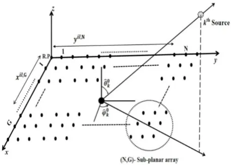
Fig. 1. Planar antenna array.

Fig. 1 introduces a planar array oriented in xoy plane and arranged as sub-planar arrays and indexed with N, G along y

planar array where n=1,…,N, g=1,…,G, has elements indexed L, I along y and x directions respectively. For any pairs (i, l), its coordinates with respect to the reference point (R.P) along y and x directions respectively are ( _),

where i=1,…,I, l=1,…,L.

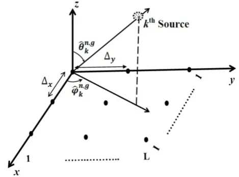
Fig. 2. Sub-Planar antenna array.

The space phase factors along x and y directions are expressed as

( ) ( ) ( ) (2)

(( ) ) (( ) ) (3)

( ) ( ) ( ) (4)

(( ) ) (( ) ) (5)

where ( ) denote the kth source estimated elevation angle and azimuth angle respectively with respect to (n, g) sub-array, and are reference displacements between neighbor elements along x and y directions within any (n, g) sub-array also and are reference displacements between neighbor sub-arrays along x and y directions respectively, and is the wavelength of the signal. The receiving model can be expressed as: [ ( )] [ _{][ ( )] [ ( )] (6)}

where the matrices, [ ( )] [ ] and [ ( )] are the receiving signal, transform factor for each sub-array, and AWGN (Additive White Gaussian Noise), respectively. They are given in subspace as follows [ _{( )] [} ( ) ( ) ( ) ( )] (7)

[ ] [ ( ) ( ) ( )] (8)

where denotes the Kronker product. So, for any (n, g) sub-array ( ) [ ] (9)

where ( ), and ( ), are symbolized as , . And: ( ) ( ) (10)

[ ( )] [ ( ) ( )] (11)

[ ( )] [ ( ) ( ) ( ) ( )] (12)

The auxiliary polarization angle is defined as γ [ ⁄ ], and the polarization phase difference is given as [ ]. We omit (n, g) for simplicity. The whole data is divided into M snapshots at each time ts second with sampling frequency fs according to Nyquist law. Then it picks up enough data r enclosed by each snapshot m with time period as short as possible. So, from (6) each receiving signal measurement value through mth subspace is given as [ ( )] [ ] ( ) [ ( )] (13)

The index m runs as m =1, 2, …, M snapshots. Therefore, the whole space-time steering data matrix can be expressed as [ ( ) ( ) ( ) ( ) ( ) ( ) ( ) ( ) ( ) ( ) ( ) ( ) ] (14)

Then [[ ( )] [ ( )] [ ( )]] (15)

where ( ), the dimension of [Z] for the kth signal is (2IL Mr). For the mth subspace data matrix can be expressed as [ ( )] [ ( ) ( ) ( ) ( ) ] (16)

For T-ESPRIT scheme the ESPRIT algorithm is used in an appropriate picked data represented in (14) for each (m) subspace given in (16). It is noted that (15) presents a parallel calculation for each subspace for the same sampling accuracy, however, the calculations load reduction and consequently saving time are achieved. The ESPRIT algorithm is based on a covariance formulation that is ̂ [ ( ) ( )] ̂ (17)

̂ [ ( ) ( )] (18)

where ̂ is the correlation matrix of the sub-array output signal matrix, ̂ is the autocorrelation matrix of the signal. The subscript (*) denotes the complex conjugate transpose. The correlation matrix of ̂ can be done for eigenvalue decomposition as follow ̂ ̂ ̂ ̂ ̂ (19)

where the eigenvalues are ordered ( )

The eigenvectors ̂ = [ ̂ ̂ ̂ ] for larger K

eigenvalues spans the signal subspace, the rest 2(I )

smaller eigenvalues ̂ [ ̂ ̂ ( )] spans the noise

Therefore, there exists a unique nonsingular matrix Q, such that

̂ [ ] [ ( ) ( )] (20)

In (13) let and be the first and the last 2L ( I -1) rows of A respectively, they differ by the factor

along the x direction. So

, where is the diagonal matrix with

diagonal elements . Consequently, ̂ and ̂ will be

the first and the last 2L (I-1)sub-matrices formed from ̂ . Then the diagonal elements of are the eigenvalues of the unique matrix _{, that satisfies}

̂ ̂ (21)

Similarly, the two 2I (L-1) sub-matrices and

consist of the rows of A numbered ( ) and

( ) respectively, differ by the space

factors along the y direction,

l=1,…,2(L-1). Then where is the diagonal

matrix with diagonal elements . Consequently, ̂ forms the 2I (L-1) two sub-matrices ̂ and ̂ . Then the

diagonal elements of , are the eigenvalues of the unique matrix _{, that satisfies}

̂ ̂ (22)

Therefore, the arrival angles ( ) for each sub-array can be calculated as

{

[( ( )

) ( ( )) ]

⁄

} (23)

_[ ( )

( )] (24)

B. Doppler Correction

The moving target echo signal is shifted by the Doppler frequency. The more accurate T-ESPRIT algorithm should consider the effect of the Doppler frequency shift due to the target movement. So,

( )

̀ (25)

( )

̀ (26)

where ̀ and ̀ are the wavelength components of the received wave into antenna plane and differ from the transmitted wavelength because of the Doppler frequency caused by the target moving velocity ⃗ [20], [21], [22]. As shown in Fig. 3, it is obvious that the wavelength ̀ and

̀ have expressions caused by the velocity components vxand vy,

̀ ( ) (27) ̀ ( ) (28)

Substituting into (25), (26), then

( )

( ) (29)

( )

( ) (30)

where

⃗ (31)

⃗ (32)

And

⃗

(33)

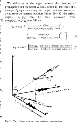
We define α as the angle between the direction of propagation and the target velocity vector ⃗, the value of α changes sign indicating the target direction toward or away from the antenna position. From (29)-(32) the arrival angles ( ) can be fine estimated from

( ( ) ( )) as follows

{[( ( )

( ⁄ ) ( ) ⃗⃗ )

( ( )

( ⁄ ) ( ( ) ⃗⃗ ) ] ⁄

} (34)

_[ ( ) ( )

( ⁄ ) ( ) ⃗⃗ ) ( ⁄ ) ( ) ⃗⃗ ] (35)

Fig. 3. Target linear velocity components into antenna plane

C. Optimal DOAE Calculation

Fig. 4. Arrangement of sub-Planar pair.

For sub-Planar pair shown in Fig. 4, the TDOA ( ) for the kth received signal is calculated as follow [23]

where is the wave velocity (3×108 m/sec) and H is the distance between any (n, g) sub-array groups as shown in Fig. 4. For the sub-planar groups shown in Fig. 5, the TDOA between group (1, 1) and group (N, G) for the kth source is denoted by , and the TDOA between group (N, 1) and group (1, G) for the kth source is denoted by .

So, from (36)

̂ (37) ̂ ₍₃₈₎

And

√( ) ( ) (39)

where are the distance between the first and last sub-array arranged along x and y directions respectively.

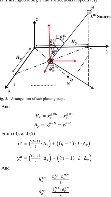
Fig. 5. Arrangement of sub-planar groups.

And

(40) (41)

From (3), and (5)

(( ) ) (( ) ) (42)

(( ) ) (( ) ) (43) And

̂ ̂ ̂ ₍₄₄₎

̂ ̂ ̂ ₍₄₅₎

Where the value of for any (n, g) sub-array group was estimated as in (34). Substitute (39-45) into (37), (38) the kth

received signal TDOA ( _{) are obtained. So, as shown}

in Fig.5 the optimal DOAE values ( ) are measured at the center of the sub-array groups which is located in the cross point of the straight lines pass through group (1, 1) and group (N, G) and through group (N, 1) and group (1, G). Thus, ( ) values can be represented in terms of

( ̂ ̂ ) as follow [23], [24]

̂ _{̂ ̂ (46)}

̂ ̂ ̂ (47) From (46), (47) the optimal DOAE values are

̂ (

) (48)

̂ _{( √( ) ( ) ) (49)}

III. SIMULATION RESULTS

Considering the 2D-DOAE process with the AWGN, the parameters are given fs = 25 MHz. Assuming total 25

temporal snapshots, pickup enclosed data r =20 times, and 200 independent Monte Carlo simulations. In order to validate the proposed method, it has been used in the planar case with number of elements, such as (I, L) = (3, 3), (N, G) = (2, 2) with displacement values

/2, with initial values of θ=45o and φ=60o. It is found that the computational load has been decreased as a result of reducing the measurement matrix dimension to [ ]

instead of [ ( )( ) ] . Table. I represents the computational time and complexity of the proposed method in term of number of flip-flops. It is obvious that the computational load has been reduced as a result of employing time subspace and spatial subspace to enable a simultaneous processing for M subspaces with each has r

snapshots for sub-array with (I, L) elements instead of processing for one space has a large number of snapshots d,

(d=Mr) snapshots for array with (IG, LN) elements.

TABLEI

COMPUTATION TIME AND COMPLEXITY COMPARISON

Algorithm

Computational

Conventional ESPRIT Proposed algorithm

time (msec) 17.7 1.14

complexity O([4d(IGLN)

2

+ 8(IGLN)3])

O([M+4r(IL)2

+8(IL)3])

Fig. 6 is plotted the RMSEs of the proposed algorithm (T-ESPRIT with spatial subspace) by dividing the planar array into two sub-planar arrays with (I, L) = (3, 3), (N, G) = (2, 2). Results shown in Fig. 6 indicate that the proposed algorithm errors are getting closer to the CRB as a result of applying subspace concept with Doppler correction. The accuracy improvement of the 2D-DOAE using proposed algorithm has been verified by comparing the resulted RMSEs with the RMSEs of 2D-Beamspace ESPRIT (DFT-ESPRIT) algorithm used in [15].

Fig. 6. RMSEs vs. SNR for the proposed (T-ESPRIT & spatial subspace) combined algorithm.

-5 0 5 10 15

10-4 10-3 10-2

SNR (dB)

R

MS

E

s

o

f

D

O

A

E

s

(

d

e

g

r

e

e

) Subspace algorithm without doppler correction_{Subspace algorithm with doppler correction}

Fig. 7. RMSEs vs. SNR for the proposed algorithm and Beam space-ESPRIT methods.

A comparison results displayed in Fig. 7 show that the errors of the proposed algorithm are less than the errors of ESPRIT algorithm in [15]. This upgrade has been realized due to the increase of DOAE accuracy when combining the T-ESPRIT with spatial subspace algorithm applying the subspace approach which decreases the errors caused by the model non-linearity effect and increases the resolution of phase deference measurement. Additionally, this improvement is due to Doppler correction which reduces the DOAE uncertainty associated with effect of the target movement.

From Table. I, it has been found that the proposed algorithm requires O(2[M+4r(IL)2+8(IL)3]) flops [25], while the conventional ESPRIT algorithm needs

O(2[4d(IGLN)2+ 8(IGLN)3]) flops. The proposed ESPRIT algorithm requires about 6% of the computational time compared with that of the classical ESPRIT algorithm.

Clearly we can figure out that the process of combining between the refined T-ESPRIT algorithm and the spatial subspace algorithm achieved success into increasing the DOAE accuracy with low computational load. Simply, the developed ESPRIT method improves the estimator performance.

IV. CONCLUSIONS

In this paper, a new ESPRIT method is developed based on the concept of subspace. Firstly, T-ESPRIT method algorithm is used to estimate DOA for each sub-array realizing time subspace concept. Secondly, T-ESPRIT DOA estimated value is corrected according to Doppler frequency resulted from target movement. Finally, the modified T-ESPRIT method is combined with TDOA algorithm to compute the optimal DOAE value which was estimated with different sub-arrays to realize spatial subspace concept. It has been found that the estimation accuracy has been increased with low computational load; also the computational time has been reduced about 94%, which consequently enhance the estimator performance.

REFERENCES

[1] Youssef Fayad, Caiyun Wang, Qunsheng Cao Alaa El-Din Sayed Hafez, “A developed ESPRIT algorithm for DOA estimation,”

Frequenz, vol.69,no. 3, pp. 263 – 269, 2015.

[2] Youssef Fayad, Caiyun Wang, Alaa El-Din Sayed Hafez, Qunsheng Cao, “Direction of Arrival Estimation Using Novel ESPRIT Method for Localization and Tracking Radar Systems,” Proceedings of the

IEEE 11th _{International Bhurban Conference on Applied Sciences &}

Technology (IBCAST), Islamabad, Pakistan, January 14–18, 2014,

pp. 396-398.

[3] Nordkvist N. and Sanyal A.K.,“Attitude Feedback Tracking with Optimal Attitude State Estimation,” American Control Conference, 2010, pp.2861-2866.

[4] Richard Roy, A. Paulraj and Thomas Kailath, “ESPRIT-Estimation of Signal Parameters via Rotational Invariance Techniques, acoustic, Speech, and signal processing,” IEEE international conference on

ICASSP, 1986, vol. 11. pp. 2495-2498.

[5] R. H. Roy, “ESPRIT-Estimation of signal parameters via rotational invariance techniques,” Ph.D. dissertation, Stanford Univ., Stanford, CA, 1987.

[6] Richard Roy and Thomas Kailath, “ESPRIT-Estimation of Signal Parameters Via Rotational Invariance Techniques,” IEEE

Transaction on acoustic, Speech, and signal processing, vol. 37,

no. 7, pp. 984-995, 1989.

[7] Z. I. Khan, R.A. Awang, A. A. Sulaiman, M. H. Jusoh, N. H. Baba, M. MD. Kamal and N. I. Khan, “Performance Analysis for Estimation of Signal Parameters via Rotational Invariance Technique (ESPRIT) in estimating Direction of Arrival for linear array antenna,” IEEE international RF And Microwave conference, Kuala Lumpur, Malaysia, December 2-4, 2008, pp.530-533. [8] Aweke N. Lemma, Alle-Jan van der Veen and Ed F. Deprettere,

“Joint Angle-Frequency Estimation using Multi-Resolution ESPRIT,”

Proceedings of the IEEE International Conference on Acoustics,

Speech and Signal Processing, 1998, vol.4, pp. 1957-1960.

[9] Gui-min Xu, Jian-guo Huang “Multi-resolution Parameters Estimation for Polarization Sensitivity Array,” IEEE International

Symposium on Knowledge Acquisition and Modeling Workshop,

KAM, 2008, pp. 180-183.

[10] Volodymyr Vasylyshyn, “Direction of Arrival Estimation using ESPRIT with Sparse Arrays,” EUMA-6th European Radar

Conference, 30 September – 2 October, Rome, Italy, 2009,

pp.246-249.

[11] Aweke N. Lemma, Alle-Jan van der Veen and Ed F. Deprettere, “Multiresolution ESPRIT Algorithm,” IEEE Transaction on signal

processing, vol. 47, no. 6, pp. 1722-1726, 1999.

[12] F. Gao, A. B. Gershman, “A generalized ESPRIT approach to direction of arrival estimation,” IEEE Signal Processing Letters, vol. 12, no. 3, pp. 254 – 257, 2005.

[13] A. L. Swindlehurst, B. Ottersten, R. Roy, and T. Kailath, “Multiple invariance ESPRIT,” IEEE Transactions on signal

processing, volume. 40, no. 4, pp.867 – 881, 1992.

[14] Jian Li and R. T. Compton, Jr., “two-dimensional angle and polarization estimation using the ESPRIT Algorithm,” IEEE

Transactions on Antennas and Propagation, vol. 40, no. 5, pp. 550 –

555, 1992.

[15] Cherian P. Mathews, Martin Haardt, Michal D. Zoltowski, “performance analysis of closed-form, ESPRIT based 2-D angle estimator for rectangular arrays,” IEEE Signal Processing Letters, vol. 3, no. 4, pp. 124 – 126, 1996.

[16] Y. Zhang, Z. Ye, X. Xu, and J. Cui, “Estimation of two-dimensional direction-of-arrival for uncorrelated and coherent signals with low complexity,” IET Radar Sonar Navigation, vol. 4, no.4, pp.507-519, 2010.

[17] Fang-Jiong Chen, Sam Kwong, Chi - Wah Kok, “ESPRIT-Like Two-Dimensional DOA Estimation for Coherent Signals,” IEEE

Transactions on Aerospace and Electronic Systems vol. 46 ,

no. 3 , pp. 1477 – 1484, 2010.

[18] Jiang Hui, Yang Gang “an improved algorithm of ESPRIT for signal DOA estimation,” International conference on industrial

control and electronics engineering, Aug 23-25, 2012, pp.317 – 320.

[19] X. Xu, Z. Ye, “Two-dimensional direction of arrival estimation by exploiting the symmetric configuration of uniform rectangular array,”

IET Radar Sonar Navigation, vol. 6, no.5, pp.307-313, 2012.

[20] F. B. BERGER, “The Nature of Doppler Velocity Measurement,”

IRE transactions on aeronautical and navigational electronics,

vol. ANE-4, no. 3, pp. 103 – 112, 1957.

[21] A. Nabavizadeh, M. W. Urban, R. R. Kinnick, and M. Fatemi, “Velocity Measurement by Vibro-Acoustic Doppler,” IEEE

Transactions on Ultrasonics, Ferroelectrics, and Frequency Control,

vol. 59, no. 4, pp. 752 - 765 , 2012.

[22] A-level Physics (Advancing Physics), http://en.wikibooks.org. , 2015.

[23] Ye Tian, Akiyoshi Tatematsu, Kazuo Tanabe, and Kiyotomi Miyajima, “Development of Locating System of Pulsed Electromagnetic Interference Source Based on Advanced TDOA Estimation Method,” IEEE Trans. electromagnetic compatibility, vol. 56, no. 6, pp.1326-1334, 2014.

[24] T. Tantisattayakul, K. Masugata, I. Kitamura, K. Kontani, “Broadband VHF sources locating system using arrival-time

-10 -8 -6 -4 -2 0 2 4 6 8 10

differences for mapping of lightning discharge process,” Journal of

Atmospheric Solar-Terrestrial Phys., vol. 67, pp. 1031–1039, 2005.

[25] Cheng Qian, Lei Huang and H.C. So “Computationally efficient ESPRIT algorithm for direction-of-arrival estimation based on Nyström method,” Signal Processing, vol. 94, pp.74-80, 2014.

Youssef Fayad (Alexandria Egypt, 4/9/1975)

received the B.S. In electronic engineering and the M.S. in communications and electronics from faculty of engineering, Alexandria University, Egypt, in 1997, 2010 respectively. He is currently in Ph.D. degree in radar system in Nanjing University of Aeronautics and Astronautics, college of electronic and information engineering, Nanjing, china. He is an IAENG Member, and a Student Member of IEEE, he is also worked as an Assistant Lecturer in Air Defense College, Egypt. Mr. Fayad research interests in antenna and radar signal processing.

Caiyun Wang was born in Shanxi, China, on

September 30, 1975. She graduated in 1996 with a B.S. degree and in 1999 with a M.S. degree. She received the Ph.D. degree in signal and information processing from Beihang University, Beijing, China, in 2008. She is currently an associate professor with the College of Astronautics , Nanjing University of Aeronautics and Astronautics (NUAA). Her major research interests are in the fields of radar automatic target recognition (RATA), radar signal processing, and adaptive signal processing, and pattern recognition.

Qunsheng Cao received his Ph.D. in electrical