B. Model of the Elevation Motion



Abstract—Multiple Rocket Launcher Systems (MLRS) are used to aim rockets to the desired elevation (pitch) and azimuth (yaw) angles in order to hit targets. In this paper, a dynamic model for an MLRS with electromechanical actuators is presented along with performance evaluation of four different friction models. The final model is simulated and the results are compared with the test data taken from the real MLRS. The results show that the proposed model is accurate within, on average, 5% of the actual system.

Index Terms—azimuth and elevation, dynamic modeling, electromechanical actuators, multiple launch rocket system.

I. INTRODUCTION

ultiple Launch Rocket Systems (MLRS) are designed based on the requirements arising from the type of ammunition and the field of operation. Constraints are imposed by the structure of the carrier vehicle and the thrust force of the ammunition. A MLRS has two degrees of freedom; elevation axis (pitch) and azimuth axis (yaw). An MLRS produced by Roketsan is shown in Fig. 1 as an example.

Fig. 1. Firing a 300 mm Rocket from Roketsan Launcher System [1]

A general schematic of an MLRS is given in Fig. 2. Rotation around the azimuth axis is done by a turntable. Although several mechanisms can be applied for rotation, the most common one is the slewing ring mechanism [2]. The slewing ring is driven by a pinion attached to a geared drive motor. A brake motor is also included for fixing the turntable during firing.

Manuscript received March 17, 2015; revised March 31, 2015. This work was supported in part by Roketsan A.Ş.

S. Sert is with Roketsan A.Ş., Elmadağ, Ankara 06780 Turkey and TOBB University of Economics and Technology, Ankara 06590 Turkey (phone: +90-536-7296411; e-mail: ssert@roketsan.com.tr).

Y. Tascioglu is with the Department of Mechanical Engineering, TOBB University of Economics and Technology, Ankara 06590 Turkey (e-mail: ytascioglu@etu.edu.tr).

Fig. 2. General Schemtic of an MLRS

The elevation table rotates with the turntable. Pitch motion around the elevation axis is achieved by using hydraulic pistons [3] or electromenhanical linear actuators [4]. In this case the elevation actuator consists of two linear actuators, two corner gearboxes, a center gearbox and an electric motor. The schematic of the elevation actuator is given in Fig. 3.

Fig. 3. Elevation Actuator

II. MATHEMATICAL MODEL OF MLRS A. Assumptions and System Definition

The mathematical model only includes the components that affect the dyamics of the system. These are; rockets, tubes, elevation table, turntable, base table, slewing ring, azimuth actuator and elevation actuator. Geometric, physical and mechanical properties of these parts are obtained from 3D models. The base table is assumed rigid and stationary, hence its mass and inertia is not modeled. For azimuth motion, the coordinate system is placed at the center of the base plate. Slewing is considered as a bearing with rigid

Dynamic Modeling of a Multiple Launch

Rocket System

Serdar Sert, Yigit Tascioglu

M

Elevation Table

Elevation Actuator

Turntable

Base Table

rings and balls. The gap between its inner and outer rings, and the gaps between balls and the rings are ignored. The turntable is placed on the slewing ring. Azimuth actuator is mounted on the turntable but the teeth of the pinion are in contact with the slewing ring. The rod ends of the elevation actuator are connected to the turntable and the elevation table via spherical bearings. In order to simplify the simulations, elevation and azimuth motions are analyzed separately [6].

B. Model of the Elevation Motion

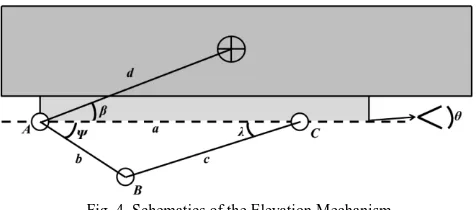
The schematics of the elevation mechanism is given in Fig. 4.

Fig. 4. Schematics of the Elevation Mechanism

The large block at the top represents the tube with rockets and the smaller block at the bottom represents the elevation table. A, B and C are revolute joints and the sign on the top block indicates the center of gravity of the two blocks combined. Variable dimensions are length (c) and inclination (λ) of the elevation actuator, and the elevation angle θ. The dashed line is the reference line showing the position when the elevation table is at 0° elevation angle.

Torque requirement from the elevation motor changes as θ varies between 0° and 60°. To model the motor torque as a function of the elevation angle, firstly, moment with respect to joint A is written as;

) sin cos(β θ) F a (λ g d

me   e (1)

where; me is the total mass of the elevation table and loaded tubes, g is the gravitational acceleration, and Fe is the force acting on the elevation actuator at joint C. Rearranging the terms to express Fe results in:

) sin cos (λ a θ) (β g d m

Fe e



 (2)

To eliminate the variables other than θ from the right hand side of (2), sin(λ) is replaced by;

c ysin( ) )

sin(   , (3)

where c can be written, by applying the law of cosines to the triangle ABC,as;





2_{  }

 b a ba

c (4)

Substituting in (2) results in an expression for Fe in terms of θ:

) sin( ) cos( 2 )

cos( 2 2













F_e e (5)

Torque applied by the elevation motor Tme is related to Fe as follows;

) (

2 _{co ce me}

ce co li

e p n n T

F 









where; p is the pitch of the linear actuator, nco and nce are the reduction ratios of the corner and center gearboxes respectively, and ηli , ηco and ηce are the efficiencies of the linear actuator, corner gearbox and center gearbox respectively. Replacing (5) in (6) and rearranging terms results in: ) 2 )( sin( ) cos( 2 )

cos( 2 2

ce co ce co li e me n n b a a b a b p d g m T





















 (7)

In order to find the angular velocity of the elevation motor dθme/dt as a function of the elevation velocity dθ/dt, firstly, (4) is differentiated.

dt d a b dt dc

c 2 sin( ) 

2   (8)

Then, the relation between the velocity of the linear actuator dc/dt and dθme/dt is written as:

dt d n n p dt dc _me ce co   2  (9)

Substituting (4) and (9) in (8) and rearranging the terms results in: dt d a b a b p a b n n dt

d _{me co ce} 

      ) cos( 2 ) sin( 2 2

2_{  }



 (10)

Equations (7) and (10) express, respectively, the torque and the angular velocity of the elevation motor as a function of the elevation angle.

C. Model of the Azimuth Motion

Fig. 5. Schematics of the Azimuth Mechanism

In order to calculate the friction force due to slewing ring, the axial force and bending moment acting on the slewing ring are determined. The axial force Fsr acting at the center of the slewing ring is;

e t

sr W W

F   (11)

where, We is the total weight of the elevation table and loaded tubes, and Wt is the weight of the turntable.

Bending moment Msr at the center of the slewing ring is; )

sin ( ) cos cos

(u  d  W w 

W

M_sr _e   _t (12)

According to [7], friction moment Msrf on the slewing ring is calculated from Fsr and Msr as;

) 4

. 4 )( 2 /

( sr sr L

srf M F D

M    (13)

where, DL is the raceway diameter, and μ is the coefficient of friction.

Slewing ring friction is affected by various parameters. Based on the empirical knowledge, the error margin is ±%25. Also, if the slewing ring is mounted on a surface with flatness deviation of 1 mm, friction moment increases by %75 [7]. If these values are applied as factors of safety, the friction moment on the slewing ring becomes;

srf

srf M

M (1.25)(1.75) (14)

During azimuth motion, torque is also required to backdrive the azimuth brake. Although the brake is released during rotation, it resists the motion due to backdriving its gearbox with a high reduction ratio. Consequently, the torque required from the aximuth motor to rotate the MLRS is;

gear gear mech

back sr

srf ma

n M n M T

 

 

( / ) (15)

where, Mback is the backdriving torque of azimuth brake, nsr is the reduction ratio between the slewing ring and the pinion, ngear and ηgear are, respectively, the reduction ratio and efficiency of the aximuth motor gearbox, and ηmech is the efficiency of the intermediate mechanical parts.

It should be noted that the inertia of the MLRS is ignored because the azimuth motion is very slow. The required torque to move against inertia is negligible compared to the friction torque.

Finally, the relation between angular velocity of the aximuth motor dθma/dt and the azimuth velocity dθa/dt is written as:

dt d n n dt

d a

gear sr

ma 

 _

(16)

III. FRICTION MODEL

The most basic approach for modeling friction in a MLRS is the simple Coulomb friction model with a single, constant coefficient of friction, which is usually estimated empirically. However, this model does not reflect the real characteristics of the system. There exist various friction models, details of which can be found in the academic literature such as [8]. The aim of this section is to find an appropriate friction model for the MLRS by implemeting the most commonly used ones to the MLRS model and comparing the simulation results with the data measured from the actual system.

Friction models are applied to the azimuth axis. Elevation angle is kept at 0° so that the unbalance load remains constant. Since the azimuth velocity is low, inertial loads are neglected and the torque requirement is assumed to be caused by friction only.

Fig. 6. Azimuth Velocity Profile (a) and Measured Motor Torque (b)

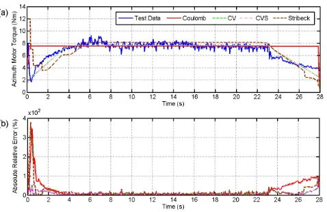
Fig. 7. Comparison of Friction Models and Test Data (a) Absolute Percent Relative Error of Friction Models (b)

with Coulomb, Coulomb+Viscous (CV), Coulomb+ Viscous+StartUp (CVS), and Stribeck friction models. More detail on the implementation of the models can be found in [9].

Fig. 7(a) shows that, only the CVS and Stribeck models simulate the beginning of the motion (i.e. 0 to 0.5 s). In the acceleration and deceleration regions all models except the Coulomb model have similar trends. The absolute relative percent error in the constant velocity region is below an acceptable 10% for all of the models (Fig. 7b).

TABLE I

IAE AND ITAE FOR FRICTION MODELS

CV CVS Stribeck

IAE 0.50 0.50 0.82

ITAE 0.40 0.40 0.67

Considering the Coulomb model as a baseline, IAE (Integral Absolute Error) and ITAE (Integral Time-Weighted Absolute Error) are calculated for the other models and given in Table 1. Although the CV and CVS models scored the same IAE and ITAE, the CV model can not simulate the stiction at the beginning of the motion. Consequently, the CVS friction model is chosen as the best alternative.

IV. RESULTS

To confirm the validity of the derived MLRS model, simulations are compared to the test data of the elevation axis, in which the motor torque is required to support the unbalance load in addition to the friction torque. During simulations, the CVS friction model is added to the elevation axis model.

Fig. 8. Comparison of Elevation Velocity of Test and Simulation (a) Absolute Percent Relative Error of Elevation Velocity (b)

The actual elevation axis is given velocity profile in Fig. 8(a). The model is tuned by iteration until the overall average of the absolute percent relative error is below 1% (Fig. 8b).

Fig. 9. Comparison of Motor Torques of Test and Simulation (a) Absolute Percent Relative Error of Elevation Motor Torque (b)

Fig. 9(a) presents the torque data of the elevation motor. It is shown that the actual motor torque is closely matched by the simulation. According to Fig. 9(b), the absolute percent relative error stays below 10% along two thirds of the motion, then raises up to 20% towards the end of the constant speed section and reaches to a maximum of 27% during deceleration. A possible explanation for this trend is that the friction characteristics change due to increasing unbalance load. However, the overall average of the absolute percent relative error remains below 5%.

V. CONCLUSION

In this paper, dynamic model of a multiple launch rocket system with electromechanical actuators is constructed and the mechanisms for azimuth and elevation are explained. Performances of four different friction models are evaluated on the azimuth axis by comparing simulation results with data measured from the actual system. The Coulomb+ Viscous+StartUp friction model is shown to be the best alternative for the application. This friction model is then implemented into the elevation axis model, which is more complicated than the azimuth axis model due to unbalance loading. It is shown, by comparing the elevation simulations with the test data, that the model is accurate within, on average, 5% of the actual system.

REFERENCES

[1] T-300 MBRL, 300 MM Multi Barrel Rocket Launcher, (2014, January 11). Available:

http://www.roketsan.com.tr/en/urunler-hizmetler/kara- sistemleri/satihtan-satiha-roket-sistemleri/t-300-cnra-300-mm-cok-namlulu-roketatar/

[2] K. Dokumacı, M. T. Aydemir, and M. U. Salamcı, “Modeling, PID Control and Simulation of a Rocket Launcher System,” in Proc.16th

International Power Electronics and Motion Control Conference and Exposition, Antalya, 2014, pp. 1518–1523.

[3] WS-2 Multiple Launch Rocket System, (2014, January 11). Available: http://www.military-today.com/artillery/ws2.htm

[4] M270 MLRS Multiple Launch Rocket System, (2014, January 11). Available: http://www.military-today.com/artillery/m270_mlrs.htm

[5] BM-21 Grad Multiple Launch Rocket System, (2014, January 11). Available: http://www.military-today.com/artillery/grad.htm

[7] Thyssenkrupp Slewing Ring Catalogue, Thyssenkrupp Rothe Erde (2015, March 10). Available:

https://www.thyssenkrupp-rotheerde.com/download/info/GWL_EN_13.08_V05W.pdf

[8] H. Olsson, K. J. Astrom, C. Caunas de Wit, M. Gafvert, P. Lischinky, “Friction Models and Friction Compensation” European Journal of Control, vol 4, no.3, pp. 176-195, 1997