Comparison of Different Heat Capacity
Approximation in Solidification Modeling
Robert Dyja, Elzbieta Gawronska, Andrzej Grosser, Piotr Jeruszka and Norbert Sczygiol
Abstract—The article presents the results of numerical mod-eling of the solidification process. We used one of the enthalpy formulations of solidification. In particular, we focused on comparing the results of calculations for various methods of the effective thermal capacity approximation used in the apparent heat capacity formulation of solidification. We have shown that the choice of one of four tested methods of approximation does not significantly affect the results and duration of the numerical simulations. Differences in the resulting temperature did not exceed a few degrees.
Index Terms—enthalpy, heat-capacity, solid-phase, solidifica-tion, computer-simulation.
I. INTRODUCTION
A
LUMINUM alloys are very interesting material widely used in industry. Modeling and computer simulation is one of the most effective methods of studying of difficult problems in foundry and metallurgical manufacture. Numer-ical simulations are use for optimization of casting produc-tion. In many cases they are a unique possible technique for carrying out of the experiments which real statement is complicated. Computer modeling allows defining the major factors for a quality estimation of alloy castings. Simulations help to investigate interaction between solidifying casting and changes of its parameters or initial conditions. That process defines a quality of casting, and a problem of adequate modeling of foundry systems, firstly, depends on solution of heat equations [1].Increasing capacity of computer memory makes it possi-ble to consider growing propossi-blem sizes. At the same time, increase precision of simulations triggers even greater load. There are several opportunities to tackle this kind of prob-lems. For instance, one can use parallel computers [2], [3], other can use accelerated architectures such as GPUs [4] or FPGAs [5], still other can use special organization of computations [6], [7], [8].
Solidification may take place at a constant temperature or in the temperature range [9]. If solidification occurs at a constant temperature, it is said then about the so-called Stefan problem or the solidification problem with zero temperatures range. At constant temperature solidify pure metals or alloys of certain specific chemical compositions, e.g., having an eutectic composition. A sharp separation of the liquid phase from solidified phase occurs in the Stefan problem. The two phases are in contact to form a solidification surface (front). Mathematical description of Stefan problem consists in the equation of heat conduction and so-called Stefan condition existing on the solidification surface. However, most of the metal alloys solidify in certain temperature ranges (so-called
Manuscript received July 9, 2015; revised July 29, 2015.
All authors work at Czestochowa University of Technology, Dabrowskiego 69, PL-42201 Czestochowa, Poland. (phone: (+48 34) 3250589; fax: (+48 34) 3250589; e-mail: [email protected]).
temperature intervals of solidification). The temperature at which the alloy starts to solidify called liquidus temperature (Tl), and the temperature at which solidification ends is called
solidus temperature (Ts). In the case of alloys with eutectic
transformation, in which the solute concentration exceeds its maximum solubility in solid phase, the temperature of the solidification end is the eutectic temperature. Analytically (rarely) and numerical (commonly) methods are used in mod-eling of solidification process. The finite elements method (FEM) is the most commonly used numerical methods, but also applies finite difference method (FDM), boundary element method (BEM), the Monte-Carlo and others.
The most important heat effect, occurring during solid-ification, is the emission of (latent) heat of solidification (L). It is also the most difficult phenomenon to numer-ical modeling. The basic division of numernumer-ical methods of solidification modeling process relates to modeling the latent heat emission. These methods can be divided into front-tracking methods and fixed-grid methods. The second group of methods are also divided into temperature formula-tions (the latent heat of solidification is considered as the temperature-dependent term of heat source) and enthalpy formulations (the latent heat of solidification is considered as the temperature-dependent term of heat capacity) [10], [11], [12], [13], [14]. In turn, the enthalpy methods are divided into the methods in which the effective heat capacity depends on the temperature and those in which the effective heat capacity depends on the enthalpy. In our article, we focused on the solidification in the temperature range solving by the finite element method with use of fixed-grid methods in enthalpy formulation. We described a comparison among the different ways of approximation of heat capacity in apparent heat capacity (AHC) formulation of solidification.
II. DESCRIPTION OF THEENTALPHYFORMULATION
Solidification is described by quasi-linear equation of heat conduction, considering a term of heat sourceq˙ as a latent heat of solidification:
∇ ·(λ∇T) + ˙q=cρ∂T
∂t (1)
By entering the following designation:
˙
s= ˙q−cρ∂T
∂t (2)
equation (1) can be written as
∇ ·(λ∇T) + ˙s= 0 (3)
h=
Z T
Tref
cρ(T)dt (4)
whereTref is the reference temperature, and calculating the
derivative with respect to the temperature:
dH
dT =cρ(T) =c
∗(T) (5)
wherec∗is the effective heat capacity. Assuming heat source equal to zero, the equation (3) can be converted to the form:
∇ ·(λ∇T) =c∗∂T
∂t (6)
All above equations form the basis of the thermal descrip-tion of solidificadescrip-tion.
A. The Enthalpy and The Effective Heat Capacity
The enthalpy is the sum of explicit and latent heat [15]. For the metal solidifying in the temperature range (Ts—Tl)
amounts to:
H =
Z T
Tref
cρs(T)dT, for T < Ts,
H =
Z Ts Tref
cρs(T)dT +
Z T
Ts (ρs(T)
dL dT +
+cρf(T)) dT, for Ts≤T ≤Tl,
(7)
H =
Z Ts Tref
cρs(T)dT +
+ρs(T)L+
Z Tl Ts
cρf(T)dT +
+
Z T
Tl
cρl(T)dT, for T > Tl
The integration of the expressions in Equation 7 gives
c∗ = cρ
s, for T < Ts,
c∗ = cρf+ρsdL
dT, for Ts≤T ≤Tl, (8)
c∗ = cρ
l, for T > Tl.
Assuming that the heat of solidification is exuded spread evenly throughout the temperature range of solidification, can write:
c∗ = cρ
s, for T < Ts,
c∗ = cρ
f+ρs
L Tl−Ts
, for Ts≤T ≤Tl, (9)
c∗ = cρ
l, for T > Tl.
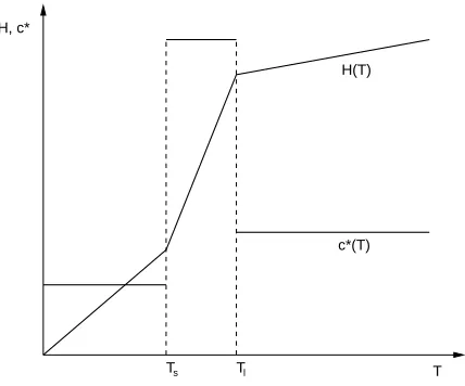
On the basis of the Equation 7 and the Equation 9 can make the following graphical comparison of the enthalpy and the effective thermal capacity distributions for alloy solidifying in the temperature range (see Figure 1).
c*(T) H, c*
H(T)
[image:2.595.320.534.52.230.2]T Ts Tl
Fig. 1. Distribution of enthalpy and effective heat capacity depending on temperature.
B. The Types of the Entalphy Formulations
There are three types of enthalpy formulations of solidifi-cation:
• basic enthalpy formulation (BEF)
∇ ·(λ∇T) = ∂H
∂t (10)
where
H(T) =
Z T
Tref
cρ dT + (1−fs(T))ρsL (11)
• apparent (or modified) heat capacity (AHC) formulation differentiate Eq. 11 with respect to temperature is ob-tained
dH
dT =cρ−ρsL dfs
dT =c
∗(T) (12)
SinceH =H(T(x, t))then
∂H ∂t =
dH dT
∂T ∂t =c
∗(T)∂T
∂t (13)
Substituting Eq. 13 to Eq. 10 is obtained
∇ ·(λ∇T) =c∗(T)∂T
∂t (14)
• source term formulation (STF)
The total enthalpy is divided into two parts in accor-dance with:
H(T) =h(T) + (1−fs)ρsL (15)
where
h(T) =
Z T
Tref
cρ dT (16)
Derivative Eq. 15 with respect to time is
∂H ∂t =
∂h ∂t −ρsL
∂fs
∂t (17)
Substituting Eq. 17 to Eq. 10 is obtained
∇ ·(λ∇T) +ρsL
∂fs
∂t = ∂h
III. APPROXIMATION OF THEEFFECTIVEHEAT CAPACITY
The effective heat capacity can be also calculated directly from the Equation 5, but in this paper, we present the results of solidification simulations using the various methods of effective heat capacity approximation.
1) Morgan method – derivative of enthalpy is replaced by a backward differential quotient
c∗=H
n−Hn−1
Tn−Tn−1 (19)
wheren−1 andn are the time levels. In some cases, however, this substitution may lead to oscillations in the solution, especially near the boundaries of the temperature range of solidification.
2) Del Giudice method – in order to remove oscillations take into account the directional cosines of temperature gradient
c∗= ∂H ∂n ∂T ∂n = ∂H ∂xi αni ∂T ∂n where
αni=
∂T ∂xi ∂T ∂n and ∂T ∂n = ∂T ∂n · ∂T ∂n 12 Hence
c∗= ∂H ∂x ∂T ∂x + ∂H ∂y ∂T ∂y + ∂H ∂z ∂T ∂z (∂T ∂x)
2+ (∂T
∂y)
2+ (∂T
∂z)
2
= H,iT,i
T,jT,j
(20)
3) Lemmon method – the temperature gradient is normal to solidification surface
c∗=
v u u u u u u t ∂H ∂x 2 + ∂H ∂y 2 + ∂H ∂z 2 ∂T ∂x 2 + ∂T ∂y 2 + ∂T ∂z 2 =
H,iH,i
T,jT,j
12
(21) 4) Comini method – the apparent heat capacity is
approx-imated by expression
c∗= 1 n ∂H ∂x ∂T ∂x + ∂H ∂y ∂T ∂y + ∂H ∂z ∂T ∂z = 1 n H,i T,i (22)
wheren is number of dimensions.
IV. NUMERICAL MODEL OF SOLIDIFICATION
Solving the partial differential equations can pass from spatial discretization through time discretization to approxi-mate solution. First, we use the finite element method.
The finite element method facilitates the modeling of many complex problems. Its wide application for founding comes
from the fact that it permits an easy adaptation of many existing solutions and technique of solidification modeling.
Computer calculations need to use discrete models, which means problems must be formulated by introducing time-space mesh. These methods convert given physical equations into matrix equations (algebraic equations). This system of algebraic equations usually contain many thousands of unknowns, that is why the efficiency of method applied to solve them is crucial.
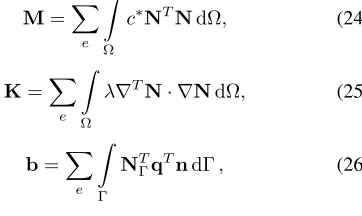
The semi-discretization of the governing equation leads to the ordinary differential equation with time derivative, given as:
M(T) ˙T+K(T)T=b(T) (23)
whereMis the capacity matrix,Kis the conductivity matrix,
T is the temperature vector and b is the right-hand side vector, whose values are calculated on the boundary condi-tions basis. The global form of these matrices is obtained by summing of coefficients for all the finite elements. The matrix components are defined for a single finite element as follows:
M=X
e
Z
Ω
c∗NTNdΩ, (24)
K=X
e
Z
Ω
λ∇TN· ∇NdΩ, (25)
b=X
e
Z
Γ
NTΓqTndΓ, (26)
whereN is a shape vector in the area Ω,NΓ is a shape
vector on the boundary Γ,n is an ordinary vector towards the boundary Γ, andq is vector of nodal fluxes.
Next, we have applied one of the one-step Θ time integration schemes [16]:
• modified Euler Backward (unconditionally stable)
(Mn+ ∆tKn)Tn+1=MnTn+ ∆tbn+1, (27)
where superscript n refers following step of computa-tions.
V. RESULTS OF THENUMERICALEXPERIMENT In the paper we considered a casting solidifying in a metal mold. The finite element mesh comprising 32 814 nodes and 158 417 elements was applied on the area of the casting and mold, as shown in Figure 2. We introduced two boundary conditions: Newton and continuity condition, for which are defined the environment temperature 400K, the heat transfer coefficient with the environment 10W/m2K−1
and the heat transfer coefficient through the separation layer 1000 W/m2K−1. The initial temperature of casting was
960K, the initial temperature of mold was 600K, the size of the time step was 0.05s.
[image:3.595.364.545.313.421.2]Material properties of the alloy (which the casting is made) and the mold are given in Tables I and II, respectively.
Figure 2 shows the distribution of temperatures in the cast-ing after 25sfor the Morgan heat capacity approximation.
Fig. 2. Temperature field after 25 s of cooling. The Finite Element mesh is also visible.
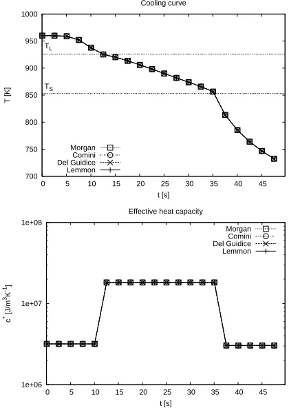
methods overlap. It is caused by a fact, that although different heat capacity approximations use different formulas, the resulting approximations are very close in values of effective heat capacity, as can be seen in a bottom part of Figure 3.
However, there is a visible difference between the heat capacity approximation formulas in calculation times. The Figure 4 shows the difference in assembly time for different methods. It is easy to notice that the Morgan method requires
700 750 800 850 900 950 1000
0 5 10 15 20 25 30 35 40 45
T [K]
t [s] Cooling curve
TS TL
Morgan Comini Del Guidice Lemmon
1e+06 1e+07 1e+08
0 5 10 15 20 25 30 35 40 45
c
* [J/m 3K -1]
t [s] Effective heat capacity
[image:4.595.75.285.453.749.2]Morgan Comini Del Guidice Lemmon
Fig. 3. A cooling curve of a point located in origin of coordinate system. The bottom plot presents change of approximate heat capacity.
TABLE I
MATERIAL PROPERTIES OF THEAL-2%CU ALLOY(SUBSCRIPTsMEANS SOLID PHASE ANDl–LIQUID PHASE)
Quantity name Unit Value
Densityρs kg/m3 2824
Densityρl kg/m3 2498
Specific heatcs J/kgK−1 1077 Specific heatcl J/kgK−1 1275 Thermal conductivity coefficientλs W/mK−1 262 Thermal conductivity coefficientλl W/mK−1 104 Solidus temperatureTs K 853
Liquidus temperatureTl K 926
Solidification temperature of pure
componentTM K 933
Eutectic temperatureTE K 821
Heat of solidificationL J/kg 390 000 Partition coefficient of solutek — 0.125
TABLE II
MATERIAL PROPERTIES OF THE MOLD
Quantity name Unit Value
Density kg/m3
7500 The specific heat J/kgK−1 620 Thermal conductivity coefficient W/mK−1 40
the least time, while the other formulas are close together in time requirement.
The results from the Figure 4 were obtained for 750 time-steps and mesh from Figure 1. On the 750th time-step the minimum solid fraction was still 0.95. This ensures that during all the calculation time in at least some fraction of finite elements the heat capacity approximation formulas were used.
VI. CONCLUSIONS
Analyzing the numerical results obtained from calculations carried out with the help of own computer program using the finite element method and the apparent heat capacity method we can draw the following remarks and conclusions:
1) The capacity formulation gives equation very similar to the equation of heat conduction; heat of solidification is hidden in the effective thermal capacity.
2) The use of any of the heat capacity approximation method does not affect the obtained result, if the solution is stable.
1000 1020 1040 1060 1080 1100 1120 1140 1160 1180
Morgan Comini Lemmon Del Guidice
Time [s]
Heat capacity approximation
[image:4.595.320.526.583.750.2]3) Using the Morgan method of heat capacity approxima-tion should be careful not to apply too small time step, because then we can get incorrect results.
4) Heat capacity approximation formulas other than Mor-gan are susceptible to give wrong results if temperature values in nodes of one finite element differs by very small values. Especially sensitive to this is the Comini method.
5) Morgan method requires the least time for calculations.
REFERENCES
[1] D. M. Stefanescu,Science and Engineering of Casting Solidification. New York: Kluwer Academic, 2002.
[2] R. Wyrzykowski, L. Szustak, and K. Rojek, “Parallelization of 2d mpdata eulag algorithm on hybrid architectures with gpu accelerators,”
Parallel Computing, vol. 40, no. 8, pp. 425–447, 2014.
[3] J. W. Kim and R. D. Sandberg, “Efficient parallel computing with a compact finite difference scheme,”Computers & Fluids, vol. 58, pp. 70–87, 2012.
[4] G. Michalski and N. Sczygiol, “Using CUDA architecture for the computer simulation of the casting solidification process,” in Proceed-ings of the International MultiConference of Engineers and Computer Scientists. Hong Kong: Lecture Notes in Engineering and Computer Science, March 2014, pp. 933–937.
[5] N. Yang, D. W. Li, J. Zhang, and Y. G. Xi, “Model predictive controller design and implementation on FPGA with application to motor servo system,”Control Engineering Practice, vol. 20, no. 11, pp. 1229–1235, 2012.
[6] E. Gawronska and N. Sczygiol,Numerically Stable Computer Simula-tion of SolidificaSimula-tion: AssociaSimula-tion Between Eigenvalues of Amplifica-tion Matrix and Size of Time Step. Springer Netherlands, 2015, pp. 17–30.
[7] ——, “Relationship between eugenvalues and size of time step in computer simulation of thermomechanics phenomena,” inProceedings of the International MultiConference of Engineers and Computer Scientists. Hong Kong: Lecture Notes in Engineering and Computer Science, March 2014, pp. 881–885.
[8] ——, “Application of mixed time partitioning methods to raise the ef-ficiency of solidification modeling,”12th International Symposium on Symbolic and Numeric Algorithms For Scientific Computing (SYNASC 2010), pp. 99–103, 2010.
[9] F. Stefanescu, G. Neagu, A. Mihai, I. Stan, M. Nicoara, A. Raduta, and C. Opris, “Controlled temperature distribution and heat transfer process in the unidirectional solidification of aluminium alloys,” Ad-vanced Materials and Structures Iv, vol. 188, pp. 314–317, 2012. [10] Q. Duan, F. L. Tan, and K. C. Leong, “A numerical study of
solidification of n-hexadecane based on the enthalpy formulation,”
Journal of Materials Processing Technology, vol. 120, no. 1-3, pp. 249–258, 2002.
[11] A. W. Date, “A novel enthalpy formulation for multidimensional solidification and melting of a pure substance,” Sadhana-Academy Proceedings in Engineering Sciences, vol. 19, pp. 833–850, 1994. [12] R. Dyja, N. Sczygiol, Z. Domanski, S. Ao, A. Chan, H. Katagiri, and
L. Xu, “The effect of cavity formation on the casting heat dissipation rate,”Iaeng Transactions on Engineering Sciences, pp. 341–347, 2014. [13] M. Famouri, M. Jannatabadi, and H. T. F. Ardakani, “Simultaneous estimations of temperature-dependent thermal conductivity and heat capacity using a time efficient novel strategy based on mega-nn,”
Applied Soft Computing, vol. 13, no. 1, pp. 201–210, 2013. [14] S. Ganguly and S. Chakraborty, “A generalized formulation of latent
heat functions in enthalpy-based mathematical models for multi-component alloy solidification systems,”Metallurgical and Materials Transactions B-Process Metallurgy and Materials Processing Science, vol. 37, no. 1, pp. 143–145, 2006.
[15] N. Sczygiol and G. Szwarc, “Application of enthalpy formulation for numerical simulation of castings solidification,” Computer Assisted Mechanics and Engineering Sciences, no. 8, pp. 99–120, 2001. [16] L. W. Wood,Practical Time-stepping Schemes. Oxford: Clarendon