A New Density-based Spatial Clustering
Algorithm for Extracting Attractive Local Regions
in Georeferenced Documents
Tatsuhiro Sakai, Keiichi Tamura,
Member, IAENG
, and Hajime Kitakami
Abstract—Nowadays, with the increasing attention being paid to social media, a huge number of georeferenced documents, which include location information, are posted on social media sites via the Internet. People have been transmitting and collecting information through these georeferenced documents. Georeferenced documents are usually related to not only personal topics but also local topics and events. Therefore, extracting “attractive” local regions associated with local topics from georeferenced documents is one of the most important challenges in different application domains. In this paper, a novel spatial clustering algorithm, called the (ǫ, σ) -density-based spatial clustering algorithm, for extracting “attractive” local regions in georeferenced documents is proposed. We defined a new type of spatial cluster called an (ǫ, σ) -density-based spatial cluster. The proposed clustering algorithm can recognize not only semantically-separated but also spatially-separated spatial clusters. To evaluate our proposed clustering algorithm, geo-tagged tweets posted on the Twitter site are used. The experimental results show that the (ǫ, σ) -density-based spatial clustering algorithm can extract “attractive” local regions as(ǫ, σ)-density-based spatial clusters.
Index Terms—density-based clustering, spatial cluster, DB-SCAN, social media, local topic extraction.
I. INTRODUCTION
I
N recent years, with widespread use of smart phones equipped with a GPS, as well as the increasing interest in social media, a huge number of georeferenced documents, which include location information, are posted on social media sites through the Internet. People have been transmit-ting and collectransmit-ting information related to location through georeferenced documents [1], [2]. Georeferenced documents are usually closely related not only to personal topics but also to local topics and events. Therefore, extracting local topics and events from georeferenced documents [3] contribute to different geo-location application domains such as, local area marketing, tourism informatics, and local topic recommen-dation.Researchers, who are interested in knowledge discovery on georeferenced documents posted on social media sites, have made a great effort to tackle the new challenges that extract local topics and events from georeferenced documents. Dense regions, in which many georeferenced documents including a keyword are posted, are the hot areas of local topics related
This work was supported in part by Hiroshima City University Grant for Special Academic Research (General Studies).
T.Sakai is with Faculty of Information Sciences, Hiroshima City Univer-sity, 3-4-1, Ozuka-Higashi, Asa-Minami-Ku, Hiroshima 731-3194 Japan, corresponding e-mail: [email protected]
K.Tamura and H.Kitakami are with Graduate School of Information Sciences, Hiroshima City University, 3-4-1, Ozuka-Higashi, Asa-Minami-Ku, Hiroshima 731-3194 Japan, e-mail:{ktamura, kitakami} @hiroshima-cu.ac.jp
to the keyword. For example, Crandall et al. [4] developed an algorithm for identifying hot sites and landmarks from geo-tagged photos posted on the Flickr site, one of the most fa-mous photo-sharing sites. Sakaki et al. [5] focused on tweets posted on the Twitter site about typhoons and earthquakes to estimate a typhoon’s trajectory and an earthquake’s epicenter using dense regions.
We have been developing a new spatial clustering algo-rithm, which extracts “attractive” local regions that are dense regions in which many georeferenced relevant documents including some keywords relevant to local topics are posted. To extract “attractive” local regions, we define a new type of spatial cluster called a(ǫ, σ)-density-based spatial cluster. An (ǫ, σ)-density-based spatial cluster is not only spatially-separated but also semantically-spatially-separated from other spa-tial clusters. Thus, (ǫ, σ)-density-based spatial clusters are closely related to local topics and events.
The main contributions of this study are as follows:
• To extract(ǫ, σ)-density-based spatial clusters, we
pro-pose a new spatial clustering algorithm for georefer-enced documents, called the(ǫ, σ)-density-based spatial clustering algorithm, which is a natural extension of DBSCAN [6]. DBSCAN is a basic density-based spatial clustering algorithm and is based on neighborhood density and recognizes an area those density is higher than that of the other areas. However, it does not take account of similarities between the contents of geo-referenced documents. The (ǫ, σ)-density-based spatial clustering algorithm can recognize(ǫ, σ)-density-based spatial clusters, which are both semantically-separated and spatially-separated from other spatial clusters.
• To recognize semantically-/spatially-separated clusters
as(ǫ, σ)-density-based spatial clusters, we define a new similarity measurement for georeferenced documents on social media sites. In social media sites, people usually post georeferenced documents that are short messages including a local topic and event. Therefore, if geo-referenced documents include a same keyword, which are similar each other, the georeferenced documents are similar each other. On the basis of this concept, we define the new similarity measurement based on keyword-based Simpson’s coefficient.
• To evaluate the proposed spatial clustering algorithm,
local topics.
The remainder of this paper is organized as follows. In Section 2, related work is reviewed. In Section 3, the(ǫ, σ )-density-based spatial cluster is defined. In Section 4, the (ǫ, σ)-density-based spatial clustering algorithm is described. In Section 5, the results of an evaluation using tweets posted on Twitter are presented. Finally, some concluding remarks are given in Section 6.
II. RELATEDWORK
The popularization of smart phones equipped with a GPS has opened up entirely-new types of data on social media sites. That is georeferenced data, which includes its posted location (e.g., geo tag, address, and landmark name) as well as its posted time. People on social media sites are referred to as sensors that observe real world happening around them. In other words, considering people on social media sites as sensors, georeferenced data is like sensor data that observes topics and events in the real world [7].
Since the use of the Internet has become widespread, topic detection and tracking in documents on the Internet [8] has been one of the most attractive research topics in many kinds of application domain. Above all, in social media era, we face new types of documents, called georeferenced documents which are a kind of georeferenced data and include location information. For example, on the Twitter site, which is a micro-blogging service site, geo-tagged tweets are georeferenced documents.
The most significant impact on many studies related to our work is DBSCAN, a density-based spatial clustering al-gorithm [6], [9]. The shapes of spatial clusters in geo-spatial data usually vary in form. Even some spatial clusters are completely surrounded by (but not connected to) a different cluster. To extract arbitrarily shaped clusters, density-based spatial clustering algorithms focuses on high dense regions in data space, separated by regions of a lower density. DBSCAN and subsequent studies were applied to studies on extracting specific areas related to local topics and events from geo-spatial data.
Tamura et al. [10] proposed a novel density-based spa-tiotemporal clustering algorithm, which can extract spatially and temporally-separated clusters in georeferenced docu-ments. Their proposed algorithm integrates spatiotemporal criteria into DBSCAN to separate spatial clusters temporally. Kisilevich et al. [11] also proposed P-DBSCAN, a new density-based spatial clustering algorithm based on DB-SCAN, for analysis of attractive places and events using a collection of geo-tagged photos. They defined a new density according to the number of people in the neighborhood. Our work is close to these studies. However, P-DBSCAN and the density-based spatiotemporal clustering algorithm cannot recognize semantically-separated spatial clusters.
There are some studies on clustering techniques for ex-tracting topics and events, which focused on geo-tagged tweets posted on the Twitter site and image-data posted on the Flickr sites. Watanabe et al. [12] identified locations that are currently attracting attention. Lee et al. [13] developed a method of detecting local events using spatial partitions. They separate the entire area into sub-areas using a Voronoi diagram. Their method recognizes the sub-areas in which the
gdp ε
gdp ε
gd1
gd2
gd3
gd4
gd1
gd2
gd4
gd3
σ
feature vector space
gdp
ሺகǡሻ ൌ ͵
[image:2.595.319.508.58.212.2]க ൌ Ͷ
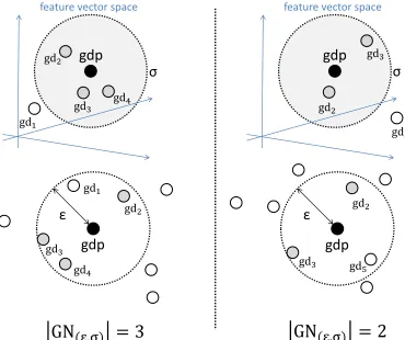
Fig. 1. Example of definition 1.
number of posted tweets is increasing. Jaffe et al. [14] devel-oped a spatial clustering algorithm for geo-tagged image data posted on the Flickr site. The spatial clustering algorithm is hierarchical and based on location information. Rattenbury et al. [15] also proposed an identification method of event places for geo-tagged image data posted on the Flickr site. Their method also can predict the contents of events using tag data. Yanai et al. [16] applied k-means to clustering geo-tagged image data. Kim et al. [17] introduced mTrend, which constructs and visualizes spatiotemporal trends of topics, named “topic movements.” These studies only focus on spatial clustering using location information, however our study focus not only spatially-separated statical clustering but also semantically-separated spatial clustering.
III. (ǫ, σ)-DENSITY-BASEDSPATIALCLUSTER
In this section, the definitions of (ǫ, σ)-density-based spatial criteria and (ǫ, σ)-density-based spatial cluster are presented.
A. Density-based Spatial Criteria
In the density-based spatial clustering algorithms, spatial clusters are dense regions separated from the regions of lower density. In other words, regions with a high density of data points are spatial clusters, whereas areas with a low density are not. The key idea of the density-based spatial clustering algorithms are that, for each data point of a spatial cluster, the neighborhood of a user-defined radius has to contain at least a minimum number of points; that is, the density in the neighborhood has to exceed some predefined threshold.
In DBSCAN, theǫ-neighborhood of a data point is defined as documents in the neighborhood of a user-defined given radiusǫ. In the ǫ-neighborhood of a data point in a spatial cluster has to contain at least minimum number of data points. In this study, a data point is a georeferenced document and the definition of ǫ-neighborhood of a georeferenced document is extended. We define the(ǫ, σ)-neighborhood of a georeferenced document to extract the semantically similar neighbors of a georeferenced document.
Definition 1 ((ǫ, σ)-neighborhoodGN(ǫ,σ)(gdp)) The
feature vector space
ሺகǡሻ ൌ ͵
ε ε
feature vector space
σ σ
ଷ ଵ
ଶ
ସ
ଵ
ଷ
ଶ
ସ
ଶ
gdp gdp
ଶ ହ
ହ ଷ
ଷ
ሺகǡሻ ൌ ʹ
[image:3.595.71.256.56.211.2]gdp gdp
Fig. 2. Example of definition 2 and definition 3.
denoted byGN(ǫ,σ)(gdp), is defined as
GN(ǫ,σ)(gdp) ={gdq∈GDS|dist(gdp, gdq)≤ǫ and sim(gdp, gdq)≥σ}, (1)
where the function dist returns the distance between geo-referenced documentgdp and georeferenced documentgdq, and the functionsimreturns the similarity betweengdpand
gdq. The functionsim is explained in the next section.
An example of the ǫ-neighborhood of gdp is shown on the left side of Fig. 1. Theǫ-neighborhood ofgdpis a set of georeferenced documents that exist withinǫfromgdp. In this example, there are four georeferenced documents in the ǫ -neighborhood ofgdp. An example of the(ǫ, σ)-neighborhood of gdp is shown on the right side of Fig. 1. The (ǫ, σ )-neighborhood ofgdpis a set of georeferenced documents ex-isting within distanceǫfromgdpand the similarity between each georeferenced document andgdpis more than a value of
σ. In this example, there are three georeferenced documents,
GN(ǫ,σ)(gdp) ={gd2, gd3, gd4}. A georeferenced document gd1is withinǫfromgdp; however, it is not inGN(ǫ,σ)(gdp),
because the similarity betweengd1andgdpis less than than
a value ofσ.
Definition 2 (Core/Border Georeferenced Document) A document gdp is called a core georeferenced document if there are at least a minimum number of georeferenced documents, M inDoc, in the (ǫ, σ)-neighborhood
GN(ǫ,σ)(gdp) (GN(ǫ,σ)(gdp) ≥ M inDoc). Otherwise,
(GN(ǫ,σ)(gdp) < M inDoc), gdp is called a border
georeferenced document.
Suppose that M inDoc is set to three. A georeferenced document gdp in the left side of Fig. 2 is a core georef-erenced document, because there are three documents in
GN(ǫ,σ)(gdp). A georeferenced document gdp in the right
side of Fig. 2 is a border georeferenced document because the number of documents inGN(ǫ,σ)(gdp)is less thanM inDoc.
Definition 3 ((ǫ, σ)-density-based directly reachable) Suppose that a georeferenced document gdq is the (ǫ, σ )-neighborhood of gdp. If the number of georeferenced documents in the(ǫ, σ)-neighborhood ofgdpis greater than or equal toM inDoc, i,e., isGN(ǫ,σ)(gdp)≥M inDoc,gdq
is(ǫ, σ)-density-based directly reachable fromgdp. In other
ଵ
ଶ
ଷ
ହ
ସ
Fig. 3. Example of definition 4 and definition 5.
words, georeferenced documents in the(ǫ, σ)-neighborhood of a core georeferenced document are (ǫ, σ)-density-based directly reachable from the core georeferenced document.
On the left side of Fig. 2, document gdp is a core geo-referenced document, because GN(ǫ,σ)(gdp) ≥ M inDoc.
Georeferenced documentsgd2,gd3andgd4are in the(ǫ, σ
)-neighborhood of gdp. These three documents are (ǫ, σ )-density-based directly reachable from gdp. On the other hand, on the right side of Fig. 2, document gdp is a border georeferenced document, i.e., is notGN(ǫ,σ)(gdp)≥ M inDoc. These two georeferenced documents are not(ǫ, σ )-density-based directly reachable fromgdpalthough georefer-enced documentgd2andgd3are in the(ǫ, σ)-neighborhood
ofgdp.
Definition 4 ((ǫ, σ)-density-based reachable) Suppose that there is a georeferenced document sequence (gd1, gd2, gd3,· · ·, gdn) and the (i + 1)-th georeferenced document gdi+1 is (ǫ, σ)-density-based directly reachable
from the i-th georeferenced document gdi. The georeferenced document gdn is (ǫ, σ)-density-based reachable fromgd1.
An example of an(ǫ, σ)-density-based reachable is shown Fig. 3. IfM inDoc= 3,gd2 is(ǫ, σ)-density-based directly
reachable fromgd1 andgd3 is (ǫ, σ)-density-based directly
reachable from gd2. The georeferenced document gd3 is
(ǫ, σ)-density-based reachable fromgd1. On the other hand, gd5 is not(ǫ, σ)-density-based reachable fromgd3, i.e.,gd2
is not(ǫ, σ)-density-based directly reachable fromgd3.
Definition 5 ((ǫ, σ)-density-based connected) Suppose that georeferenced documents gdp and gdq are (ǫ, σ)-density-based reachable from document gdo. If
N D(ǫ,σ)(gdp) ≥ M inDoc, we denote that gdp is (ǫ, σ
)-density-based connected togdq.
An example of an(ǫ, σ)-density-based reachable is shown in Fig. 3. In this figure,gd3is(ǫ, σ)-density-based reachable
fromgd1andgd5is(ǫ, σ)-density-based reachable fromgd1.
At this time,gd3 is(ǫ, σ)-density-based connected togd5.
B. Definition of Cluster
[image:3.595.361.491.69.168.2]reachable from the core georeferenced documents. A(ǫ, σ )-density-based spatial cluster is defined as follows.
Definition 6 ((ǫ, σ)-density-based spatial cluster)
An (ǫ, σ)-density-based spatial cluster (DSC) in a georeferenced document set GDS satisfies the following restrictions:
(1) ∀gdp, gdq ∈ GDS, if and only if gdq is (ǫ, σ
)-density-based reachable from gdp, gdq is also in
DSC.
(2) ∀gdp, gdq ∈ DSC, gdp is (ǫ, σ)-density-based
connected togdq.
Even if gdp and gdq are border georeferenced documents,
gdpandgdqare in a same(ǫ, σ)-density-based spatial cluster if gdpis(ǫ, σ)-density-based connected togdq.
IV. (ǫ, σ)-DENSITY-BASEDSPATIALCLUSTERING ALGORITHM
In this section, the proposed (ǫ, σ)-density-based spatial clustering algorithm is described.
A. Data Model
Let gdi denote the i-th georeferenced document in
GDS = {gd1,· · ·, gdn}; then,gdi consists of three items:
gdi =< texti, pti, pli>, where texti is the content (e.g., title, short text message, and tags), pti is the time when the geo-spatiotemporal document was posted, andpli is the location where gdi was posted or is located (e.g., latitude and longitude).
B. Algorithm
The algorithm of(ǫ, σ)-density-based spatial clustering is shown in Algorithm 1. In this algorithm, the function IsClus-teredchecks whether documentgdpis already assigned to a spatial cluster. Then, the functionGetNeighborhoodreturns the(ǫ, σ)-neighborhood of georeferenced documentgdp. For each georeferenced document gdp in GDS, the following steps are executed. Ifgdpis a core georeferenced document according to Definition 2, it is assigned to a new spatial cluster, and all the neighbors are queued to a candidate queue
CQfor further processing. The function MakeNewCluster makes a new spatial cluster. The processing and assignment of georeferenced documents to the current spatial cluster con-tinue untilCQis empty. The next georeferenced document is dequeued fromCQ. If the dequeued georeferenced document is not already assigned to the current spatial cluster, it is so assigned to the current spatial cluster. Then, if the (ǫ, σ )-neighborhood of the dequeued georeferenced document are queued to CQ using the functionEnNniqueQueue, which puts input georeferenced documents intoCQif they are not already inCQ.
C. Keyword-based Similarity Function
Letdtidenote all words intextiofi-th georeferenced doc-ument:dti={wi,1, wi,2,· · ·, wi,nw(i)}, wherewi,j∈W,W is a set of all words including in {text1, text2,· · ·, textn}.
In this study, morphological analysis extracts noun, verb and adjective phrase as words. Simpson’s coefficient has a feature
input :GDS - georeferenced document set,ǫ -neighborhood radius,σ- similarity rate,
M inDoc- threshold value output:SC - set of clusters
cid←1;
SC←φ;
fori←1 to|GDS| do
gdp←gdi∈GDS;
ifIsClustered(gdp)==f alsethen
GN←GetNeighbors(gdp,ǫ,σ); if|GN| ≥M inDocthen
stccid←MakeNewCluster(cid,gdp);
cid←cid+ 1; EnQueue(CQ,GN); whileCQis not emptydo
gdp←DeQueue(CQ);
GN← GetNeighbors(gdp,ǫ,σ); if|GN| ≥M inDocthen
EnNniqueQueue(CQ,GN); end
stccid←stccid∪gdp end
SC←SC∪stccid; end
end end returnSC;
Algorithm 1: (ǫ, σ)-Density-based Spatial Clustering Algorithm
of cosine similarity for similarity between sets. The word-based Simpson’s coefficient is defined as:
wsim(gdi, gdj) =
|dti∩dtj| |min(dti, dtj)|
. (2)
The word-based Simpson’s coefficient has drawback, when the keywords are same but several words in georeferenced documents are different. For example, suppose that there are two georeferenced documentgd1 andgd2that are related to
“Itsukushima Shrine”. If dt1 ={“Itsukushima Shrine”,
“beautif ul”, “historical”, “Hiroshima”} and dt2 = {“Itsukushima Shrine”,“wonderf ul”,“sea”,“clean”}, the similarity between two georeferenced documents is
wsim(gd1, gd2) = 1/4 = 0.25. The similarity between gd1
and gd2 is low, even though gd1 and gd2 cover the same
topic “Itsukushima Shrine.”
If georeferenced documents include a same keyword, which are be located close to each other, the georeferenced documents are similar each other. On the basis of this concept, we define the new similarity measurement based on keyword-based Simpson’s coefficient. Let keyi denote all words in dti of i-th georeferenced document: keyi = {ki,1, ki,2,· · ·, ki,nk(i)}, where ki ∈ wi, ki,j ∈ K, K is a set of all keywords including in W. The keyword-based Simpson’s coefficient is defined as:
ksim(gdi, gdj) =
|keyi∩keyj| |min(keyi, keyj)|
. (3)
Simp-TABLE I
CLUSTERING RESULTS OFDBSCAN
No Number of Tweets Range (longitude) Range (latitude) Top-5 Frequent Words
1 2173 132.34259769 - 132.5139095 34.34225649 - 34.41800308 shop, inside, today, station, come
2 288 132.301779 - 132.32664956 34.291072 - 34.317351 Miyajima, Itsukushima Shrine, Miyajimaguchi, oyster, ferry 3 170 132.4580275 - 132.4968043 34.43618755 - 34.48192577 shop, day, lunch, AEON MALL Hiroshima Gion, come
4 128 132.90427752 - 132.91733343 34.331726 - 34.348506 Tamayura, station, cat, Mr/Ms, Okonomiyaki
5 97 132.54589487 - 132.57154524 34.2343527 - 34.25657546 Yamato, museum, center, shop, noodle 6 96 132.7203672 - 132.75817651 34.4141014 - 34.43534496 Geso, person, today, set menu, shop
7 86 132.5285826 - 132.54099838 34.3442324 - 34.3628074 Mr/Ms, senaponcoro, shop, buy, seem
8 67 132.30352202 - 132.31108951 34.35173988 - 34.35770497 octopus, ball, while, open, today
TABLE II
CLUSTERING RESULTS OF THE PROPOSED SPATIAL CLUSTERING ALGORITHM(w1= 1.0ANDw2= 0.0)
No Number of Tweets Range (longitude) Range (latitude) Top-5 Frequent Words
1 97 132.4572834 - 132.46863105 34.389778 - 34.398638 shop, inside, Okonomiyaki, the head shop, Hondori 2 91 132.3154613 - 132.323433 34.2952182 - 34.304972 Miyajima, Itsukushima Shrine, Otorii, Itsukushima, Shrine
3 89 132.47242982 - 132.478453 34.39267358 - 34.401398 station, JR, Sta, Shinkansen, shop
4 47 132.4516591 - 132.45680987 34.39113274 - 34.39614078 Atomic Bomb Dome, Dome, bomb, Atomic, inside
5 32 132.9155353 - 132.919807 34.4374464 - 34.44173556 Hiroshima airport, HIJ, RJOA, lounge, ANA
6 18 132.177305 - 132.179825 34.16595235 - 34.169017 Kintaikyo, Yokoyama, the foot of the bridge, back side, cross 7 18 132.303433 - 132.310635 34.30675418 - 34.311843 Miyajima, ferry, Miyajimaguchi, JR West Japan, conger 8 15 132.31584043 - 132.31844813 34.36297389 - 34.36718941 Miyajima SA, outbound, San’you Expressway, Starbucks, coffee
TABLE III
CLUSTERING RESULTS OF THE PROPOSED SPATIAL CLUSTERING ALGORITHM(w1= 0.5ANDw2= 0.5)
No Number of Tweets Range (longitude) Range (latitude) Top-5 Frequent Words
1 58 132.47208448 - 132.47934873 34.39384782 - 34.40005438 Station, JR, Sta, Shinkansen, platform
2 41 132.4522132 - 132.45680987 34.39113274 - 34.395784 Atomic Bomb Dome, Atomic, Dome, Bomb, inside
3 34 132.3154613 - 132.32271635 34.295341 - 34.3043505 Miyajima, Otorii, Itsukushima, oyster, do
4 25 132.31876669 - 132.32147207 34.2958401 - 34.30074774 Itsukushima Shrine, Itsukushima, Shrine, Shrine, Itsukushima 5 17 132.177305 - 132.179825 34.16595235 - 34.169017 Kintaikyo, Yokoyama, the foot of the bridge, back side, Cross 6 15 132.9155353 - 132.91950762 34.4374464 - 34.44173556 Hiroshima Airport, HIJ, RJOA, Arrival, B787
7 13 132.42671107 - 132.42702243 34.37271835 - 34.37327164 SemiHard Toast, baked, one down, favor, today 8 12 132.45691723 - 132.45915413 34.40035934 - 34.40379812 Castle, Castle, beautiful, huge castle, Mizuhori
son’s coefficient and the keyword-based Simpson’s coeffi-cient. The similarity functionsim is defined as:
sim(gdi, gdj) =w1 × wsim(gdi, gdj)
+ w2×ksim(gdi, gdj), (4)
where, w1+w2 = 1.0. If w1 and w2 are set to 1.0 and
0.0 respectively, the keyword-based similarity function only use words similarities. On the other hand, If w1 andw2 are
set to 0.0 and 1.0 respectively, the keyword-based similarity function only use keywords similarities.
In the example described above, suppose that w1 = 0.5
and w2 = 0.5. The return value of wsim(gdi, gdj)is 0.25 and the return value of ksim(gdi, gdj) is 1.0. Thus, the return value of the keyword-based similarity functionsimis 0.5×0.25 + 0.5×1.0 = 0.6125. Georeferenced documents
gd1 and gd2 including the local topic of “Itsukushima
Shrine” are determined be similar each other by using a new similarity measurement.
V. EXPERIMENTALRESULTS
To evaluate the(ǫ, σ)-density-based spatial clustering algo-rithm, we used an actualGDSthat is composed of crawling tagged tweets on the Twitter site. We collected geo-tagged tweets from the Twitter site using its API. The number of tweets is 480,000. The time period is from November 2011 to February 2012. In the experiments, we compare the(ǫ, σ )-density-based spatial clustering algorithm with DBSCAN.
The parameters of DBSCAN were set to ǫ=500m,
M inDoc=5. The parameters of the (ǫ, σ)-density-based spatial clustering algorithm were set to ǫ=500m, σ=0.7,
M inDoc=5. Moreover, we used two types of the keyword-based similarity functions. One is that weight parametersw1
andw2are set to 1.0 and 0.0 respectively (called the
words-based method). The other is that weight parametersw1 and w2 are set to 0.5 and 0.5 respectively (called the
keywords-based method). We ranked the clusters on the basis of the number of tweets included in each cluster.
Table I, Table II and III show the details of extracted spatial cluster ranked in the number of tweets. These table show the number of tweets, the range of longitude and latitude of each cluster. Moreover, top 5 of frequent words in each cluster are shown, but words relevant to address such as Hiroshima and city is excluded.
Table I shows the details of extracted spatial cluster using DBSCAN. The region of cluster 1 covers the downtown of Hiroshima; however, there are many local topics in it. Fig. 4 shows the locations of tweets in clusters 1 on the geographical coordinate space. The density of posed tweets in the downtown of Hiroshima is high because there are many people there. Therefore, this region is extracted as one spatial cluster including several local topics. As a result, DBSCAN can not recognize semantically-separated spatial clusters.
Table II and III show the ranking of extracted spatial clusters using the (ǫ, σ)-density-based spatial clustering al-gorithm. Table II shows the results of the proposed clustering algorithm using the words-based method. Table III shows the results of the proposed clustering algorithm using keywords-based method. In contrast to DBSCAN, the (ǫ, σ )-density-based spatial clustering algorithm recognized multiple spatial clusters.
34.32 34.34 34.36 34.38 34.4 34.42 34.44
132.3 132.35 132.4 132.45 132.5 132.55
L
atitud
e
[image:6.595.92.244.60.155.2]Longitude clusuter 1
Fig. 4. Data plots in downtown of Hiroshima using DBSCAN.
34.39 34.395 34.4 34.405
132.45 132.46 132.47 132.48
La
tit
u
d
e
Longitude cluster 1 cluster 3 cluster 4
34.39 34.395 34.4 34.405
132.45 132.46 132.47 132.48
L
atit
u
d
e
Longitude cluster 1 cluster 2 cluster 8
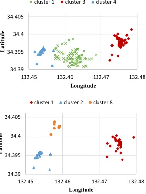
Fig. 5. Data plots in downtown of Hiroshima using the proposed spatial clustering algorithm (the upper figure is the words-based method and the lower figure is the keywords-based method).
the areas of cluster 1, cluster 2, cluster 8 are located in the downtown of Hiroshima. Fig. 5 shows the locations of tweets in extracted spatial clusters located in the downtown of Hiroshima on the geographical coordinate space.
The (ǫ, σ)-density-based spatial clustering algorithm can recognize semantically-separated spatial clusters; however cluster 1 in Table II includes local topics downtown in Hiroshima. There are many tweets related to “Okonomiyaki restaurant”, “streetcars” and “Hiroshima’s oyster.” These tweets include the same address. Table II shows the results of the words-based method. Therefore, the algorithm deter-mined these tweets are similar. On the other hand, this cluster is not extracted in the keywords-based method.
The extracted spatial clusters clusters 4 of Table II and clusters 2 of Table III, although both clusters are “Atomic Bomb Dome”, the keywords-based method is six tweets less than the words-based method. We checked six tweets manually, the topic of these six tweets is “Atomic Bomb Dome Sta”. This result indicates that the keywords-based method can recognize accurate spatial cluster compared with the words-based method.
VI. CONCLUSION
In this paper, we propose a novel spatial clustering algorithm, called the (ǫ, σ)-density-based spatial cluster-ing algorithm, for extractcluster-ing “attractive” local regions in georeferenced documents. The proposed spatial clustering algorithm can recognize not only spatially-separated but
also semantically-separated spatial clusters. To evaluate our proposed clustering algorithm, geo-tagged tweets posted on the Twitter site are used. The experimental results show that the (ǫ, σ)-density-based spatial clustering algorithm can ex-tract “atex-tractive” local regions as(ǫ, σ)-density-based spatial clusters. In our future work, we are going to develop online algorithm to extract(ǫ, σ)-density-based spatial clusters.
REFERENCES
[1] M. Naaman, “Geographic information from georeferenced social me-dia data,”SIGSPATIAL Special, vol. 3, no. 2, pp. 54–61, jul 2011. [2] S. Van Canneyt, S. Schockaert, O. Van Laere, and B. Dhoedt,
“De-tecting places of interest using social media,” inProceedings of the The 2012 IEEE/WIC/ACM International Joint Conferences on Web Intelligence and Intelligent Agent Technology - Volume 01, ser. WI-IAT ’12, 2012, pp. 447–451.
[3] H. Yang, S. Chen, M. R. Lyu, and I. King, “Location-based topic evolution,” inProceedings of the 1st international workshop on Mobile location-based service, ser. MLBS ’11, 2011, pp. 89–98.
[4] D. J. Crandall, L. Backstrom, D. Huttenlocher, and J. Kleinberg, “Mapping the world’s photos,” inProceedings of the 18th international conference on World wide web, ser. WWW ’09, 2009, pp. 761–770. [5] T. Sakaki, M. Okazaki, and Y. Matsuo, “Earthquake shakes twitter
users: real-time event detection by social sensors,” inProceedings of the 19th international conference on World wide web, ser. WWW ’10, 2010, pp. 851–860.
[6] M. Ester, H.-P. Kriegel, J. Sander, and X. Xu, “A density-based algorithm for discovering clusters in large spatial databases with noise,” inSecond International Conference on Knowledge Discovery and Data Mining, E. Simoudis, J. Han, and U. M. Fayyad, Eds. AAAI Press, 1996, pp. 226–231.
[7] M. F. Goodchild, “Citizens as voluntary sensors: Spatial data infras-tructure in the world of web 2.0,”International Journal of Spatial Data Infrastructures Research, vol. 2, pp. 24–32, 2007.
[8] J. Allan, R. Papka, and V. Lavrenko, “On-line new event detection and tracking,” inProceedings of the 21st annual international ACM SIGIR conference on Research and development in information retrieval, 1998, pp. 37–45.
[9] J. Sander, M. Ester, H.-P. Kriegel, and X. Xu, “Density-based cluster-ing in spatial databases: The algorithm gdbscan and its applications,”
Data Mining and Knowledge Discovery, vol. 2, no. 2, pp. 169–194, jun 1998.
[10] K. Tamura and T. Ichimura, “Density-based spatiotemporal clustering algorithm for extracting bursty areas from georeferenced documents,” inProceedings of the IEEE International Conference on System, Man, and Cybernetics, SMC 2013, 2013, pp. 2079-2084.
[11] S. Kisilevich, F. Mansmann, and D. Keim, “P-dbscan: a density based clustering algorithm for exploration and analysis of attractive areas using collections of geo-tagged photos,” in Proceedings of the 1st International Conference and Exhibition on Computing for Geospatial Research & Application, ser. COM.Geo ’10, 2010, pp. 38:1–38:4. [12] K. Watanabe, M. Ochi, M. Okabe, and R. Onai, “Jasmine: a real-time
local-event detection system based on geolocation information propa-gated to microblogs,” inProceedings of the 20th ACM international conference on Information and knowledge management, ser. CIKM ’11, 2011, pp. 2541–2544.
[13] R. Lee and K. Sumiya, “Measuring geographical regularities of crowd behaviors for twitter-based geo-social event detection,” inProceedings of the 2nd ACM SIGSPATIAL International Workshop on Location Based Social Networks, ser. LBSN ’10, 2010, pp. 1–10.
[14] A. Jaffe, M. Naaman, T. Tassa, and M. Davis, “Generating summaries and visualization for large collections of geo-referenced photographs,” inProceedings of the 8th ACM international workshop on Multimedia information retrieval, ser. MIR ’06, pp. 89–98.
[15] T. Rattenbury, N. Good, and M. Naaman, “Towards automatic extrac-tion of event and place semantics from flickr tags,” inProceedings of the 30th annual international ACM SIGIR conference on Research and development in information retrieval, ser. SIGIR ’07, pp. 103–110. [16] K. Yanai, K. Yaegashi, and B. Qiu, “Detecting cultural differences
using consumer-generated geotagged photos,” in Proceedings of the 2nd International Workshop on Location and the Web, ser. LOCWEB ’09, 2009, pp. 12:1–12:4.
[image:6.595.96.245.189.386.2]