Controllability of Linear Time-invariant Dynamical
Systems with Fuzzy Initial Condition
Bhaskar Dubey, Raju K. George
Abstract—In this paper, we investigate controllability prop-erty of the linear time-invariant systems of the form x˙ = Ax(t) +Bu(t)with fuzzy initial condition x(t0) in(E1)n and control u(t) ∈ (E1)m, where A, B, are n×n, n×m real matrices, respectively,t0 ≥0, and (E1)n denotes the set of all n−dimensional vectors of fuzzy numbers on R. We establish sufficient conditions for the controllability of such systems. Examples are given to substantiate the results obtained.
Index Terms—Fuzzy dynamical systems, Controllability, Fuzzy-number, Fuzzy-state
I. INTRODUCTION
I
N most of the physical applications we do not havethe exact value of the initial condition from which the dynamical system begins to evolve. This could be due to the fact that the precise measurement of the data could be costly or practically impossible. If the error in estimation of the initial states are not too random, they can be defined by fuzzy sets or fuzzy numbers. Similarly, the desired final state can also be modelled as a fuzzy set. Thus, the problem of steering an initial state of a system to a desired final state in
Rn, will essentially become a problem of steering a
fuzzy-state to another fuzzy-fuzzy-state in(E1)n.
Controllability of fuzzy dynamical control systems is a very important concept in the design of fuzzy systems. Broadly fuzzy systems are classified mainly in three cate-gories, namely pure fuzzy systems in which the dynamics of the fuzzy system is governed by a fuzzy differential equation, T-S fuzzy systems and fuzzy logic systems which uses fuzzifiers and defuzzifiers. Controllability of fuzzy systems has been explored by many authors, for example, Cai and Tang [2], Ding and Kandel ([3], [4]), S. S. Farinwata et al. [8], Y. Feng et el. [9], M.M. Gupta et al. [11]. Recently, Biglarbegian et al. [1] have studied the accessability and controllability properties of T-S fuzzy logic control sys-tems by using differential geometric and Lie-algebraic tech-niques. In [5], the authors introduced the concept of fuzzy-controllability, a concept weaker than fuzzy-controllability, for the systems of typex˙ =Ax(t)+Bu(t), x(0) =X0∈(E1)nand
established sufficient conditions for such systems to be fuzzy-controllable. In [9], the authors studied a concept of quasi-controllability for the fuzzy dynamical systems described by linear fuzzy differential equations.
In this paper, we consider linear time-invariant systems with fuzzy initial condition and establish results on
control-Manuscript received March 25, 2013; revised August 8, 2013. This work was supported by IIST-ISRO fellowship granted by Dept. of Space (Govt. of India).
Bhaskar Dubey is currently a doctoral student at the Department of Mathematics, Indian Institute of Space Science and Technology, Trivandrum, Kerala, 695547 India, e-mail: ([email protected]).
Raju K. George is a professor at the Department of Mathematics, Indian Institute of Space Science and Technology, Trivandrum, Kerala, 695547 India, e-mail: ([email protected])
lability properties of the system. The results in this paper can be regarded as the extension of some of the results in [5] and [9]. Firstly, the concept of controllability developed in this paper is stronger than the concept of fuzzy-controllability established in [5], that is, controllability implies fuzzy-controllability. Secondly, in [9] the authors assumed the
initial condition to be in Rn, whereas we establish our
results by assuming the initial condition to be in (E1)n,
a much wider class than Rn. Furthermore, we prove that
the controllability of the pair (A∗, B∗) obtained by flip
operations (for flip operations, see Remark III.2 and [5],[15])
on the matrix pair(A, B)is equivalent to the controllability
of the pair(A, B)and the pair(|A|,|B|), together.
The organization of the paper is as follows: In Section
II, we state preliminary definitions and results on the
fuzzy system theory. In Section III, we briefly describe
the evolution of solutions of linear time-invariant systems
with fuzzy initial condition. In SectionIV, we establish the
controllability results for linear time-invariant systems with
fuzzy initial condition. In Section V, some examples are
given to illustrate the results obtained. Finally, we conclude
the paper in SectionV I.
II. PRELIMINARIES
Let Rn, and Rn
+ denote the set of all n-dimensional
real vectors and n-dimensional non-negative real vectors,
respectively. Given a real matrix A, |A| denotes the matrix
of the size as that of A and whose entries are the absolute
values of the corresponding entries inA.E1 denotes the set
of all fuzzy numbers onR.
Definition II.1. By a fuzzy number onR, we mean a mapping µ:R→[0,1]with the following properties:
(i) µis upper semi continuous.
(ii) µ is fuzzy convex, that is, µ(αx + (1 − α)y) ≥
min(µ(x), µ(y))for all x, y∈R.
(iii) µ is normal, that is, there exists x0 ∈ R such that
µ(x0) = 1.
(iv) Closure of the support ofµ is compact, that is,cl(x∈ R:µ(x)>0) is compact inR.
For everyµ∈E1, anα-level set orα-cut ofµis denoted
byµα or[µ]
α. Forα∈(0,1], it is defined as follows:
µα={x:µ(x)≥α}.
Forα= 0, the 0-cut ofµis defined as the closure of union
of all non zeroα-cuts ofµ. That is:
µ0= ∪ α∈(0,1]
µα.
It can be easily shown that for everyµ∈E1,µαis a closed
lower and upperα−cut of µ, respectively.
We can easily see that a fuzzy number is characterized by
the endpoints of the intervals µα. Thus a fuzzy number µ
can be identified by a parameterized triple
{(µα, µα, α)|, α∈[0,1]}.
The following Lemma due to Goetschel and Voxman [10] provides a characterization of fuzzy numbers.
Lemma II.2. (Goetschel and Voxman [10]) Assume thatI= [0,1], and a:I→Rand b:I→Rsatisfy the conditions:
(a) a:I→Ris a bounded increasing function.
(b) b:I→Ris a bounded decreasing function.
(c) a(1)≤b(1)
(d) For 0 < k ≤ 1, limα→k−a(α) = a(k) and
limα→k−b(α) =b(k)
(e) limα→0+a(α) =a(0) andlimα→0+b(α) =b(0)
Thenµ:R→I defined by
µ(x) = sup{α|a(α)≤x≤b(α)}
is a fuzzy number with parametrization given by
{(a(α), b(α), α)|0 ≤ α ≤ 1}. Moreover, if µ : R → I is a fuzzy number with parametrization given by
{(a(α), b(α), α)|0 ≤ α ≤ 1}, then functions a(α) and b(α)satisfy conditions(a)−(e).
Given two vectors of fuzzy numbers X0 =
[X01, X02, . . . , X0n]T, X1 = [X11, X12, . . . , X1n]T in
(E1)n, we say X0 ≤ X1 if µ
X0i(·) ≤µX1i(·), 1 ≤i ≤n
and X0 = X1 if µX0i(·) = µX1i(·), 1 ≤ i ≤ n, where
µX0i(·), µX1i(·) are the membership functions of X0i,
X1i, respectively. Arithmetic fuzzy addition and scalar
multiplication in E1 are defined by using the extension
principle [7]. Letu, v∈E1 andβ∈R.
(u+v)(x) = sup
x=y+z
min(u(y), v(z)), x∈R
(βu)(x) =
{
u(xβ)} if β6= 0 ˜
0 if β= 0,
where˜0∈E1 is defined as follows
˜
0(x) =
{
1 if x= 0
0 if x6= 0.
Let the symbol Pk(R) denote the family of all non empty
convex, compact subsets ofR.
Definition II.3. The Hausdorff metric on Pk(R) is defined
as
d(A, B) =inf{²|A⊂N(B, ²)and B⊂N(A, ²)}, (1)
whereA,B∈Pk(R)and N(A, ²) ={x∈Rn|kx−yk< ²
for some y∈A},N(B, ²)is similarly defined.
We can define a metric onE1 by using Hausdorff metric.
DefineD:E1×E1→R+∪ {0}by
D(u, v) = sup
0≤α≤1
d(uα, vα),
wheredis the Hausdorff metric defined onPk(R).
Definition II.4. A mapping F : T = [a, b] → E1 is differentiable at t0 ∈ T if there exists a F˙(t0) ∈ E1 such
that the limits
lim h→0+
F(t0+h)−F(t0)
h ,hlim→0+
F(t0)−F(t0−h)
h ,
exist and equal to F˙(t0). Here the limits are taken in the metric(E1, D).
Suppose the parametric form ofF(t)is represented by
F(t) ={(F1(t, α), F2(t, α), α) :α∈[0,1], t∈T}.
The Seikkala [13] derivativeF˙(t)of a fuzzy function F(t) is defined by
˙
F(t) ={( ˙F1(t, α),F˙2(t, α), α) :α∈[0,1], t∈T} (2)
provided that the above equation defines a fuzzy number.
III. EVOLUTION OF SOLUTIONS OF TIME-INVARIANT
FUZZY DYNAMICAL SYSTEMS
Since we are interested in the controllability of the fol-lowing system:
{
˙
x(t) =Ax(t) +Bu(t)
x(t0) =X0,
(3)
where A and B are the n×n, and n×m real matrices
respectively, X0 ∈(E1)n, the input u(t)∈(E1)m for each
t ∈ [t0, t1] and u(·) is fuzzy-integrable (see [12],[13]) in [t0, t1]. Therefore, it is important to understand the structure of the solutions of (3). We will now briefly describe the evolution of the solutions of the system (3). The fuzziness in the control and initial condition makes the system (3) a fuzzy dynamical control system. Thus, it is clear that
state of the system at any time t ∈ [t0, t1], starting from
the initial state X0, belongs to (E1)n, that is, x(t) =
[x1(t), x2(t), . . . , xn(t)]T in (E1)n. We now introduce new variables which we shall use throughout this paper.
xα(t) := [xα1(t), xα2(t), . . . , xαn(t)]T
xα(t) := [xα
1(t), xα2(t), . . . , xαn(t)] T,
where [xα
k(t), x α
k(t)] is the α-cut of xk(t) for
1 ≤ k ≤ n. uα(t) and uα(t) are similarly
defined. We denote xα
∗(t) := [xα(t), xα(t)]T :=
[xα
1(t), xα2(t), . . . , xαn(t), x1α(t), xα2(t), . . . , xαn(t)]T a column vector of size2n.uα
∗(t)and[u(t)]αare similarly defined.
Using these variables we construct a 2n−dimensional
system following the idea suggested in [13] to study the evolution of system (3).
Lemma III.1. For α∈(0,1], letxαk(t) = [xαk(t), xα k(t)]be
theα-cut ofxk(t)for1≤k≤nanduαj(t) = [u α
j(t), uαj(t)]
be the α−cut of uj(t) for 1 ≤ j ≤ m then the evolution
of system (3) is described by the following 2n−differential equations:
˙
xα
k(t) =min((Az+Bw)k :zi∈[xαi(t), xαi(t)],
wj ∈[uαj(t), uαj(t)]) ˙
xα
k(t) =max((Az+Bw)k :zi∈[xαi(t), xαi(t)],
wj ∈[uαj(t), uαj(t)])
xαk(t0) =xα0k xαk(t0) =xα0k,
where 1 ≤ k ≤ n, and (Az +Bw)k = Σni=1akizi +
Σm
j=1bkjwj is the kthrow of Az+Bw.
Proof:A detailed proof of the above Lemma is given in [6]. However, we sketch the brief outline of the proof. The
Seikkala [13] derivativex˙(t)of the fuzzy processx:R+→
(E1)n is given by[ ˙x
k(t)]α= [ ˙xαk(t),
˙
xα
k(t)],α∈(0,1]and
1≤k≤n. On the other hand, by using extension principle
it can be shown that theα−cut of thekthrow from R.H.S. of
(3) is given by[min(Az+Bw)k, max(Az+Bw)k], where
zi ∈ [xαi(t), xαi(t)]for 1≤i ≤n, and wj ∈[ujα(t), uαj(t)]
for 1≤j≤m. Hence the lemma is proved.
Remark III.2. By using the above Lemma, the evolution of system (3) can be given by a system in a compact form as described below (see also Xu et el. [15], Dubey and George [5]):
Forα∈[0,1],x˙α
∗(t) =A∗xα∗(t) +B∗u∗α(t),xα∗(t0) =X0α∗ in which A∗ and B∗ are defined as follows:
(i) If A has all its entries non-negative thenA∗=M and B∗=N, where
M =
[ A 0
0 A
]
, N =
[ B 0
0 B
]
i.e,M is a block diagonal matrix of size2n×2nandN is a block diagonal matrix of size2n×2m. We denote M = [mij],1 ≤ i, j ≤ 2n and N = [nij],1 ≤ i ≤ 2n,1≤j ≤2m. Furthermore the symbol ”mij ←→
mkl”means that the entry inithrow andjthcolumn of
M is swapped by the entry inkthrow andlthcolumn of
M, and vice versa.”nij←→nkl”is similarly defined. (ii) If A has some of its entries negative then A∗ is obtained by the following flip operations on the entries ofM.
mij←→mi(j+n) if16j6nandmij<0,
mij←→mi(j−n) ifn < j62nand mij<0.
(iii) If B has some of its entries negative then B∗ is
obtained by the following flip operations on the entries ofN.
nij←→ni(j+m) if16j6m andnij <0,
nij←→ni(j−m) ifm < j 62mand nij<0. (iv) Ifu(t)∈Rmis a crisp vector instead of being a vector
of fuzzy numbers, thenB∗ can be taken asN and in this caseuα
∗(t) = [u(t), u(t)]T.
The flip operations in Remark III.2 are illustrated by an example in the Appendix B.
IV. MAINRESULTS
In this section, we establish some controllability results for the system (3). Before proving the main results we will briefly state some controllability results for the crisp systems which we shall use in establishing the controllability results for the fuzzy dynamical systems. Consider the linear time-invariant system x˙(t) = Ax(t) +Bu(t), x(t0) =x0 ∈Rn,
where A, B are n×n, n×m real matrices, respectively.
The system is completely controllable during time interval [t0, t1]or the pair(A, B)is controllable during[t0, t1]if any of the following conditions hold (see [14]):
(i) Controllability GrammianW(t0, t1)defined by
W(t0, t1) = ∫ t1
t0
Φ(t0, τ)BBTΦT(t0, τ)dτ
is non-singular, where Φ(t, τ) denotes the transition
matrix for the systemx˙(t) =Ax(t).
(ii) No eigenvector of AT lies in the kernel of BT (PBH
Test).
(iii) Rank of controllability matrix
[B|AB|A2B|. . .|An−1B] =n.
We will now define the controllability for the fuzzy system (3).
Definition IV.1. (Controllability) The system(3) with fuzzy initial condition x(t0) = X0 ∈ (E1)n is said to be controllable to a fuzzy-stateX1∈(E1)n att1(> t0)if there exists a fuzzy-integrable controlu(t)∈(E1)mfort∈[t0, t1]
such that the solution of system(3)with this control satisfies x(t1) =X1.
Remark IV.2. A concept of fuzzy-controllability, weaker than the controllability defined in the Definition IV.1, was introduced in [5]. In fuzzy-controllability, we do not require x(t1) = X1 instead one looks for a control u(t) ∈ (E1)m
with which the solution of system(3) satisfiesx(t1)≤X1.
We will now give sufficient conditions for the controlla-bility of fuzzy dynamical system (3). If the pair(A∗, B∗)is
controllable, whereA∗ andB∗ are obtained by the process
defined in Remark III.2 of Section 3, then a control u(·)
which steers a statex0 inR2n to a desired state x1 inR2n
during time interval[t0, t1] is given by
u(t),η(t, t0, t1, x0, x1)
:=B∗TΦ∗T(t0, t)W∗−1(t0, t1)[Φ∗(t0, t1)x1−x0],
whereΦ∗(t, τ)denotes the transition matrix for the system
˙
x(t) = A∗x(t) and W∗(t0, t1) is the controllability
Gram-mian for the systemx˙(t) =A∗x(t) +B∗u(t).
Theorem IV.3. The system (3) with fuzzy initial condition X0 ∈ (E1)n is controllable to X1 ∈ (E1)n during time interval[t0, t1] if
(i) The Pair(A∗, B∗)is controllable.
(ii) The function u(·), characterized by [u(t)]α = [uα(t), uα(t)], where uα(t), uα(t) are defined by [uα(t), uα(t)]T := η(t, t0, t1, Xα
0∗, X1α∗), belongs to Em.
Proof: LetX0 be the initial fuzzy-state at time t0 and
X1 be the prescribed fuzzy-state at time t1. The dynamics
of the system (3), under the assumptions whenx(t)∈(E1)n andu(t)∈(E1)m, is given by the following levelwise set of
equations:
˙
xα
∗(t) =A∗xα∗(t) +B∗uα∗(t), α∈(0,1] (5)
Using condition(i)it follows that for eachα∈(0,1], there exists a control u˜α∗(t) :=η(t, t0, t1, X0α∗, X1α∗) with which the solution of (5) with initial crisp state xα∗(t0) = X0α∗
satisfies xα∗(t1) = X1α∗. Condition (ii) now implies that
there exists a functionu˜(·)such thatu˜(t)∈(E1)m for each
t ∈ [t0, t1] and [˜uα(t),u˜α(t)]T = η(t, t0, t1, X0α∗, X1α∗).
Sinceu˜α∗(t)is integrable in[t0, t1], therefore ∫t1 t0 u˜
∫t1 t0 u˜
α(t)are well defined, which implies thatu˜(t)is
fuzzy-integrable in [t0, t1] (see [13]). Hence u˜(t) is a
fuzzy-controller with which the solution of (3) with fuzzy initial condition x(t0) = X0 satisfies x(t1) = X1. Hence system
(3) with initial condition X0 is controllable to X1 during
[t0, t1].
Remark IV.4. The condition (ii) of Theorem IV.3 inherently states that controllability of system(3) not only depends on matrices A and B but also on initial and final fuzzy-states, whereas crisp-controllability of system (3) depends only on matricesAandB. Therefore, given any arbitrary initial state X0∈(E1)n it may not be possible to control the system to
an arbitrary state X1 ∈(E1)n. However, if the initial state
is crisp, that is,X0∈Rn then the set of all reachable fuzzy
states fromX0can be characterized more precisely by using a result due to Feng et el. [9][Theorem 3.4]. Thus we have the following theorem.
Theorem IV.5. The fuzzy control systemx˙ =Ax(t) +Bu(t)
with the arbitrary initial condition x0 ∈Rn can be steered
to any fuzzy state in the admissible controllable state subset
(E1
0)n of (E1)n if and only if the pair (A∗, B∗) is control-lable. And the admissible controllable state subset (E1
0)n of
(E1)n is given by:
(E10)n ={V ∈(E1)n|V1−V1∈ ∩
t0≤t≤t1
(Ψ(t))−1Rm+ and
d dα
( Vα
−Vα )
∈ ∩
t0≤t≤t1
(Ψ∗(t))−1R2+m,
(6)
α∈(0,1],} (7)
whereΨ(t),Ψ∗(t)are defined as follows:
Ψ(t) =|B|TΦT|A|(t1, t)W1−1(t1, t0)
where Φ|A|(t, s)is the transition matrix for the systemx˙ =
|A|xand W1(t1, t0)is defined by W1(t1, t0) =
∫ t1
t0
Φ|A|(t1, s)|B||B|TΦT|A|(t1, s)ds.
Ψ∗(t) =|B∗|TΦT|A∗|(t1, t)W2−1(t1, t0),
whereΦ|A∗|(t, s)is the transition matrix for the systemx˙ =
|A∗|xand W2(t1, t0) is defined by W2(t1, t0) =
∫ t1
t0
Φ|A∗|(t1, s)|B∗||B∗|TΦT|A∗|(t1, s)ds.
Proof: It can be shown that the controllability of the pair (A∗, B∗) is equivalent to the controllability of pair
(|A∗|,|B∗|)(see Appendix A). Now the proof follows along the similar lines of the proof of Theorem3.4of Feng et al.[9].
We will now provide a closed form formula for the steering fuzzy control that can be applied to the systems of type (3)
with the matrices A, B having non-negative entries. For a
matrixA,A≥0, we mean that all the entries ofAare
non-negative. When A ≥0 and B ≥0, we have the following
result.
Theorem IV.6. LetA, B≥0in system(3)andW(t0, t1)is non singular then a fuzzy-controller, which steers an initial
fuzzy-stateX0∈(E1)n to a desired fuzzy-state X1∈(E1)n during time interval[t0, t1], is given by
u(t) =BTΦT(t0, t)W−1(t0, t1)(Φ(t0, t1)X1f −X0) (8)
providedX1f ∈Enwithα-level sets given by[X1f]
α= [X1α+
Φ(t1, t0)(Xα
0 −X
α
0), X1α−Φ(t1, t0)(X0α−X
α
0)].
Proof: Under the conditionA, B ≥0, the evolution of the system (3) with the control given in (8), is given by the following set of levelwise decomposed linear differential equations.(see Remark III.2)
˙
xα(t) =Axα(t) +Buα(t) ˙
xα(t) =Axα(t) +Buα(t)
xα(t0) =Xα
0 xα(t0) =Xα
0,
(9)
whereα ∈(0,1]. Using (8), uα(t) anduα(t) are obtained as below.
uα(t) =BTΦT(t0, t)W−1(t0, t1)(Φ(t0, t1)Xf1
α
−Xα
0), uα(t) =BTΦT(t
0, t)W−1(t0, t1)(Φ(t0, t1)Xf1
α
−X0α).
The solution of system (9) is given by following two
equations:
xα(t) = Φ(t, t0)X0α+
∫ t
t0
Φ(t, τ)Buα(τ)d(τ) (10)
xα(t) = Φ(t, t0)Xα
0 + ∫ t
t0
Φ(t, τ)Buα(τ)d(τ) (11)
From (10) we have,
xα(t1) = Φ(t1, t0)X0α+
∫ t1
t0
Φ(t1, τ)Buα(τ)d(τ)
= Φ(t1, t0)X0α+
∫ t1
t0
Φ(t1, τ)BBTΦT(t0, τ)
W−1(t0, t1)(Φ(t0, t1)Xf1
α
−Xα
0)d(τ)
= Φ(t1, t0)X0α+
Φ(t1, t0)W W−1(Φ(t0, t1)X1fα−Xα
0)
=Xf1
α
−Φ(t1, t0)(X0α−X
α
0) =X
α
1 (12)
Similarly from (11) we can show that
xα(t
1) =Xf1
α
+ Φ(t1, t0)(X0α−X
α
0) =X1α (13)
Equations (12) and (13) together imply that x(t1) = X1.
Hence system (3) with the control u(·) given in (8) steers
X0 toX1 during time interval [t0, t1].
Remark IV.7. If A, B ≥0 then the controllability of pair
(A∗, B∗) is equivalent to the controllability of the pair
(A, B). In general, checking the controllability conditions for the pair(A∗, B∗)is computationally inefficient due to the fact that the sizes ofA∗andB∗are twice that of the original matrices A and B, respectively. However, alternatively, the controllability of the pair (A∗, B∗) can be checked in an efficient way as expressed by the following result.
V. NUMERICALEXAMPLES
In this section, we provide examples which demonstrate controllability of time-invariant systems with fuzzy initial condition. Example V.1, V.2 apply to Theorem IV.6 and Theorem IV.3, respectively.
Example V.1. Let
˙
x(t) =x(t) + 2u(t)
and x(0) = X0 and x(1) = X1, where X0 and X1 are in
E1 and are defined as follows:
X0(s) =
{
ee−1−14s2 |s| ≤ 1
2
0 |s| ≥ 12 ,
X1(s) =
{
ee−4−4s2 |s| ≤2
0 |s| ≥2.
In the setting of above example, we haveΦ(t, τ) =et−τand
W(0,1) = 2(1−e2). Using equation(8)the fuzzy-controller,
which steers the initial fuzzy state X0 to target fuzzy state X1 during time-interval[0,1], is given by
u(t) = e
−t
(1−e2)[e
−1X1f −X0],
where the fuzzy number Xf1 is defined as follows:
∀α∈(0,1],[Xf1]α= [X1α+e(X0α−X
α
0), X1α−e(X0α−X
α
0). The propagated state at time t = 1 (Fig. 1d) coincides with the desired target state (Fig. 1b). In Fig. 2, lower
−2.50 −1.5 −0.5 0.5 1.5 2.5 0.2
0.4 0.6 0.8 1
(a) Initial state at t=0
−2.50 −1.5 −0.5 0.5 1.5 2.5 0.2
0.4 0.6 0.8 1
(b) Desired target state att= 1
−2.50 −1.5 −0.5 0.5 1.5 2.5 0.2
0.4 0.6 0.8 1
(c) System-state att= 3/4
−2.50 −1.5 −0.5 0.5 1.5 2.5 0.2
0.4 0.6 0.8 1
[image:5.595.304.546.69.167.2](d) System-state att= 1
Fig. 1: Initial, target and propagated states of the system
and upper cuts of the control and system-states are plotted corresponding to α=.5. It can be seen in the figure (2b) that [X0].5 is steered to[X1].5 during time-interval [0,1].
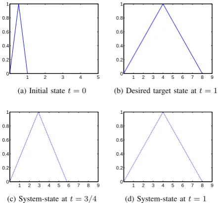
Example V.2. Let
˙
x(t) =−x(t)−2u(t)
and x(0) = X0 and x(1) = X1, where X0 and X1 are in
E1 and are defined as follows:
0 0.2 0.4 0.6 0.8 1 −0.4
−0.2 0 0.2 0.4
time
.5−cut values of the control
upper values of α−cuts (for α=.5)
lower values of α−cuts (for α=.5)
(a) Control plot forα=.5
0 0.2 0.4 0.6 0.8 1 −1.5
−1 −0.5 0 0.5 1 1.5
time
.5−cut values of the states
upper values of α−cuts (for α=.5)
lower values of α−cuts (for α=.5)
(b) State plot forα=.5
Fig. 2: Control and state plots forα=.5during[0,1]
X0(s) = {
2s 0≤s≤ 12
2−2s 12 ≤s≤1 ,
X1(s) = { s
4 0≤s≤4
2−s4 4≤s≤8.
In this case, the evolution of system is given by the following level-wise equations:
( ˙ xα(t)
˙
xα(t)
)
=
(
0 −1
−1 0
) ( xα(t)
xα(t)
)
+
(
0 −2
−2 0
) ( uα(t)
uα(t)
) .
Using Theorem IV.3, the fuzzy-controller u(·) which steers X0toX1during time-interval[0,1], is given by the following α-cut representation:
[u(t)]α=[−1.399et+e−t(1.1238α−1.349),
−1.399et+e−t(−1.1238α+ 1.349)]. (14)
It is clear from Fig. 3 that the initial fuzzy-stateX0is steered
1 2 3 4 5
0 0.2 0.4 0.6 0.8 1
(a) Initial statet= 0
1 2 3 4 5 6 7 8 9
0 0.2 0.4 0.6 0.8 1
(b) Desired target state att= 1
1 2 3 4 5 6 7 8 9
0 0.2 0.4 0.6 0.8 1
(c) System-state att= 3/4
1 2 3 4 5 6 7 8 9
0 0.2 0.4 0.6 0.8 1
[image:5.595.358.497.218.272.2](d) System-state att= 1
Fig. 3: Initial, target and propagated states of the system
[image:5.595.59.280.443.649.2] [image:5.595.316.538.488.694.2]0 0.2 0.4 0.6 0.8 1 −5
−4 −3 −2 −1
time
.5−cut values of the control
upper values of α−cuts (for α=.5)
lower values of α−cuts (for α=.5)
(a) Control plot forα=.5
0 0.2 0.4 0.6 0.8 1 0
2 4 6 8
time
.5−cut values of the states
upper values of α−cuts (for α=.5)
lower values of α−cuts (for α=.5)
[image:6.595.48.291.69.167.2](b) State plot forα=.5
Fig. 4: Control and state plots forα=.5 during[0,1]
VI. CONCLUSION
In this article, a new concept of controllability, a concept sharper than the fuzzy-controllability (see [5]), is introduced and sufficient conditions are established for the control-lability of linear time-invariant systems with fuzzy initial conditions. The results obtained are seemingly important for the controllability of systems with uncertain parameters like initial condition. Furthermore, we feel that the results can be extended to time-varying systems by using some of the results in [9]. Also, the results can be further generalized to the systems with uncertain plant parameters by considering
the matrices A and B to be fuzzy. Obviously, the present
investigation enriches our knowledge about controllability of such systems.
APPENDIXA PROOF OF THELEMMAIV.8
Proof: Assume that pair (A∗, B∗) is controllable. We want to show that(A, B)and(|A|,|B|)are also controllable. We will prove it by the method of contradiction. Suppose first
that the pair (A, B)is not controllable, then by P BH test
of controllability, there exists a non-zero vectorv∈Rnsuch
that
ATv=λv andBTv= 0. (15)
Define a vectorw= [v, v]T, then from (15) we have
A∗Tw=λw andB∗Tw= 0. (16)
By PBH test, the last equation implies that the pair(A∗, B∗) is not controllable contrary to the assumption. Similarly, if the pair (|A|,|B|)is not controllable then there exists a non
zero vector v∈Rn such that
|A|Tv=λv and|B|Tv= 0. (17)
Now, by takingw= [v,−v]T, (16) follows from (17), which
is again a contradiction.
Conversely, assume that(A, B)and(|A|,|B|)are
control-lable, we want to show that pair (A∗, B∗) is controllable.
Suppose(A∗, B∗)is not controllable, then there exists a non zero vectorx= (x1, x2, . . . , xn, xn+1, . . . , x2n)∈R2nsuch that
A∗Tx=λx andB∗Tx= 0. (18)
Now define a vector v = (v1, v2, . . . , vn) ∈ Rn such that
vi =xi+xn+i for eachi= 1,2, . . . , n. Then, from (18) it follows that
ATv=λv andBTv= 0. (19)
The last equation is contrary to the fact that pair(A, B)is
controllable. Hence the lemma.
Remark A.1. Following closely the proof given above, it can also be shown that pair (|A∗|,|B∗|) is controllable if and only if the pair(A, B)and the pair(|A|,|B|)are both controllable.
APPENDIXB
ILLUSTRATIONS OF THE FLIP OPERATIONS
Example B.1. Let
A=
[
−1 2
2 −1
] , M =
−1 2 0 0
2 −1 0 0
0 0 −1 2
0 0 2 −1
ThenA∗ is given by
A∗=
0 2 −1 0
2 0 0 −1
−1 0 0 2
0 −1 2 0
InA∗, the negative entriesm11,m22,m33,m44of the matrix M are flipped bym13,m24,m31and m42, respectively.
REFERENCES
[1] M. Biglarbegian, A. Sadeghian, W. Melek, “On the accessibil-ity/controllability of fuzzy control systems,”Information Science, Vol. 202, pp. 58-72, 2012.
[2] Z. Cai and S. Tang, “Controllability and robustness of T-fuzzy control systems under directional disturbance,”Fuzzy Sets and Systems, Vol. 115, pp. 279-285, 2000.
[3] Z. Ding and A. Kandel, “On the controllability of fuzzy dynamical systems (I),” Journal of Fuzzy Mathematics, Vol. 8(1), pp. 203-214, 2000.
[4] Z. Ding and A. Kandel, “On the controllability of fuzzy dynamical systems (II),” Journal of Fuzzy Mathematics, Vol. 8(2), pp. 295-306, 2000.
[5] Bhaskar Dubey and Raju K. George, “Estimation of controllable initial fuzzy states of linear time-invariant dynamical systems,” Communica-tions in Computer and Information Science, Springer, Vol. 283, pp. 316-324, 2012.
[6] Bhaskar Dubey and Raju K. George, “A note on the evolution of solutions of a system of ordinary differential equations with fuzzy initial conditions and fuzzy-inputs,”Journal of Uncertain Systems, Accepted for publication, July-2013.
[7] D. Dubois, H.Prade, “Towards fuzzy differential calculas. Part 3,”Fuzzy Sets and Systems, Vol. 8, pp. 225-233, 1982.
[8] S. S. Farinwata and G. Vachtsevanos, “Survey on the controllability of fuzzy logic systems,”Proceedings of32thIEEE Conference on Decision
and Control, pp. 1749-1750, 1993.
[9] Y. Feng, L. Hua, “On the quasi-controllability of continuous-time dynamic fuzzy control systems,”Chaos, Solitons&Fractals, Vol. 30 (1), pp. 177-188, 2006.
[10] R. Goetschel, W. Voxman, “Elementary calculus,” Fuzzy Sets and Systems, Vol. 18, pp. 31-43, 1986.
[11] M. M. Gupta et al., “Controllability of fuzzy control systems,”IEEE Transactions on Systems, Man, and Cybernetics, Vol. 16, pp. 576-582, 1985.
[12] O. Kaleva, “Fuzzy differential equations,”Fuzzy Sets and Systems, vol. 24, pp. 301-317, 1987.
[13] S. Seikkala, “On the fuzzy initial value problem,”Fuzzy Sets and Systems, Vol. 24, pp. 319-330, 1987.
[14] F. Szidarovszky, A.Terry Bahil, “Linear system theory,” CRC Press, 1998.
![Fig. 4: Control and state plots for α = .5 during [0, 1]](https://thumb-us.123doks.com/thumbv2/123dok_us/471988.545403/6.595.48.291.69.167/fig-control-state-plots-a.webp)
