Simultaneous Plant and Controller Optimization Based on Non-smooth Techniques

Simultaneous Plant and Controller Optimization

Based on Non-smooth Techniques

Ngoc Minh Dao, and Dominikus Noll

Abstract—We present an approach to simultaneous design optimization of a plant and its controller. This is based on a bundling technique for solving non-smooth optimization prob-lems under nonlinear and linear constraints. In the absence of convexity, a substitute for the convex cutting plane mechanism is proposed. The method is illustrated on a problem of steady flow in a graph and in robust feedback control design of a mass-spring-damper system.

Index Terms—Robust control, Hankel norm, system with tunable parameters, nonlinear optimization, steady flow.

I. INTRODUCTION

I

N modern control system, desirable closed-loop charac-teristics include stability, speed, accuracy, and robustness and depend on both structural and control specifications. Traditionally, structural design with its drive elements pre-cedes and is disconnected from controller synthesis, which may result in a sub-optimal system. In contrast, optimizing plant structure and controller simultaneously may lead to a truly optimal solution. We therefore propose design methods which allow to optimize various elements such as system structure, actuators, sensors, and the controller simultane-ously.

Here we focus on simultaneous optimization of certain plant and controller parameters to achieve the best perfor-mance for a closed-loop system with constraints. This leads to a complex nonlinear optimization problem involving non-smooth and non-convex objectives and constraints. Suitable optimization methods are discussed to address such prob-lems.

Consider a stable LTI state-space control system

G: (

δx=Ax+Bu y=Cx+Du

where δx represents x˙(t) for continuous-time systems and x(t+ 1) for discrete-time systems, and where x ∈ Rnx _is the state vector,u∈Rmthe control input vector, andy∈Rp the output vector. Our interest is the case in which system Gis placed in a control system containing actuators, sensors and a feedback controller K, and matrices A, B, C, D and controller K depend smoothly on a design parameter x

varying inRnor in some constrained subset ofRn. Denoting by Tw→z(x) the closed-loop performance channel w →z, this brings to the optimization program

minimize kTw→z(x)k subject to x∈Rn,

K=K(x)assures closed-loop stability (1)

Manuscript received July 15, 2013.

N. M. Dao is with the Department of Mathematics and Informatics, Hanoi National University of Education, Vietnam. Email: minhdn@hnue.edu.vn.

N. M. Dao and D. Noll are with the Institut de Math´ematiques, Universit´e de Toulouse, France. Email: noll@mip.ups-tlse.fr.

Here standard choices ofk · kinclude theH∞-normk · k∞, the H2-norm k · k2, or the Hankel norm k · kH which is

discussed in more detail in the sections III and VI. Solving (1) leads to non-smooth optimization problems.

II. APROXIMITY CONTROL ALGORITHM

Bundle methods are currently among the most effective ap-proachs to solve non-smooth optimization problems. In these methods, subgradients from past iterations are accumulated in a bundle, and a trial step is obtained by a quadratic tangent program based on information stored in the bundle. In the absence of convexity, tangent planes can no longer be used as cutting planes, and a substitute has to be found. A so-phisticated management of the proximity control mechanism is also required to obtain a satisfactory convergence theory. We will show in which way these elements can be assembled into a successful algorithm.

For the purpose of solving the problem (1), we present here a non-smooth algorithm for general constrained optimization programs of the form

minimize f(x)

subject to c(x)60

Ax6b

(2)

where x ∈ Rn is the decision variable, and f and c are

potentially non-smooth and non-convex, and where the linear constraints are gathered inAx6band handled directly.

Expanding on an idea in [15, Section 2.2.2], we use a progress function at the current iteratex,

F(·,x) = max{f(·)−f(x)−νc(x)+, c(·)−c(x)+},

where c(x)+ = max{c(x),0}, and ν > 0 is a fixed parameter. It is easy to see that F(x,x) = 0, where either the left branch f(·)−f(x)−νc(x)+ or the right branch c(·)−c(x)+ in the expression ofF(·,x)is active at x, i.e.,

attains the maximum, depending on whetherxis feasible for

the non-linear constraint or not.

Setting P = {x ∈ Rn : Ax 6 b}, it follows from [16,

Theorem 6.46] that the normal cone toP atx is given by

NP(x) ={A⊤η:η>0, η⊤(Ax−b) = 0}.

We remark therefore that if x∗ is a local minimum of

program (2), it is also a local minimum of F(·,x∗) on P,

and then 0 ∈ ∂1F(x∗_,

x∗) +A⊤η∗ for some multiplier

η∗ _{> 0 with η}∗⊤_(A

x∗ −b) = 0. The symbol ∂1 here

stands for the Clarke subdifferential with respect to the first variable. Indeed, ifx∗ is a local minimum of (2) then

c(x∗_{)60, A}

x∗ 6b, and so for y in a neighborhood ofx∗

we have

F(y,x∗) = max{f(y)−f(x∗), c(y)}

>f(y)−f(x∗_{)>0 =F(x}∗_,

This implies that x∗ is a local minimum ofF(·,x∗) onP,

and therefore0∈∂1F(x∗_,

x∗) +NP(x∗). We now present

the following algorithm for computing solutions of program (2).

Algorithm 1

_.

Proximity control with downshift

Parameters: 0 < γ <eγ <1,0< γ <Γ<1,0< q <∞,

0< c <∞,q < T <∞.

1: Initialize outer loop. Choose initial iterate x1 with

Ax16b and matrixQ1 =Q⊤₁ with−qI Q1 qI.

Initialize memory element τ1♯ such that Q1+τ

♯

1I ≻0. Putj= 1.

2: Stopping test. At outer loop counterj, stop the

algo-rithm if0∈∂1F(xj_,

xj)+A⊤ηj, for a multiplierηj >0

withηj⊤_(A

xj−b) = 0. Otherwise, goto inner loop.

3: Initialize inner loop. Put inner loop counterk= 1and

initializeτ1=τj♯. Build initial working model

F1(·,xj) =g0⊤j(· −xj) +1₂(· −xj)⊤Qj(· −xj),

whereg0j ∈∂1F(xj,xj).

4: Trial step generation. At inner loop counter k find

solutionyk of the tangent program

minimize Fk(y,xj) +τ₂kky−xjk2

subject to Ay6b,y∈Rn.

5: Acceptance test. If

ρk = F(y k_,

xj)

Fk(yk_, xj)

>γ,

putxj+1 =yk (serious step), quit inner loop and goto

step 8. Otherwise (null step), continue inner loop with step 6.

6: Update working model. Generate a cutting plane

mk(·,xj) =ak+gk⊤(· −xj)at null stepyk and counter

kusing downshifted tangents. Compute aggregate plane m∗

k(·,xj) =a∗k+g∗⊤k (· −xj)atyk, and then build new

working modelFk+1(·,xj).

7: Update proximity control parameter. Compute

sec-ondary control parameter

e ρk =

Fk+1(yk,xj)

Fk(yk_, xj)

and put

τk+1= (

τk ifρek <eγ, 2τk ifρek >eγ.

Increase inner loop counterk and loop back to step 4.

8: UpdateQj and memory element. UpdateQj →Qj+1

respectingQj+1= Q⊤j+1 and−qIQj+1qI. Then store new memory element

τ_j♯₊₁= (

τk if ρk<Γ,

1

2τk if ρk>Γ.

Increaseτ_j♯₊₁ if necessary to ensureQj+1+τj♯+1I≻0. Ifτ_j♯₊₁ > T then re-set τ_j♯₊₁ =T. Increase outer loop counterj and loop back to step 2.

Convergence theory of Algorithm 1 is discussed in [7], [10] and based on these results, we can prove the following theorem.

Theorem 1: Supposef andc in program (2) are

lower-C1 functions such that the following conditions hold:

(a) f is weakly coercive on constraint set Ω ={x∈Rn:

c(x)60, Ax6b}, i.e., if xj ∈Ω,kxjk → ∞, then

f(xj_{)is not monotonically decreasing.}

(b) cis weakly coercive onP, i.e., ifxj∈P,kxjk → ∞,

thenc(xj_{)is not monotonically decreasing.}

Then the sequence of serious iterates xj ∈P generated by

Algorithm 1 is bounded, and every accumulation point x∗

of thexj satisfies x∗∈P and0∈∂1F(x∗,x∗) +A⊤η∗ for

some multiplierη∗_{>0 withη}∗⊤_(A

x∗−b) = 0.

An immediate consequence of Theorem 1 is the following

Corollary 2: Under the hypotheses of the theorem, every

accumulation point of the sequence of serious iterates gen-erated by Algorithm 1 is either a critical point of constraint violation, or a Karush-Kuhn-Tucker point of program (2).

Proof: Suppose x∗ is an accumulation point of the

sequence of serious iterates generated by Algorithm 1. Ac-cording to Theorem 1 we have0∈∂1F(x∗_,

x∗) +NP(x∗).

By using [4, Proposition 9] (see also [5, Proposition 2.3.12]), there exist constantsλ0, λ1 such that

0∈λ0∂f(x∗_{) +λ1∂c(x}∗_{) +N}

P(x∗),

λ0>0, λ1>0, λ0+λ1= 1. If c(x∗_{) > 0 then ∂1F(x}∗_,

x∗) = ∂c(x∗), and therefore 0 ∈ ∂c(x∗_{) +N}

P(x∗), which means that x∗ is a critical

point of constraint violation. In the case ofc(x∗_{)60, if}

x∗

fails to be a Karush-Kuhn-Tucker point of (2), thenλ0must equal0, and so 0 ∈ ∂c(x∗_{) +N}

P(x∗). We obtain thatx∗

is either a critical point of constraint violation, or a Karush-Kuhn-Tucker point of program (2).

In the absence of convexity, proving convergence to a single Karush-Kuhn-Tucker point is generally out of reach, but the following result gives nonetheless a satisfactory answer for stopping of the algorithm.

Corollary 3: Under the hypotheses of the theorem, for

everyε > 0 there exists an index j0(ε) ∈ N such that for every j > j0(ε), xj is within ε-distance of the set L of

critical pointsx∗ in the sense of the theorem.

Proof: By the fact that our algorithm assures always

xj −xj+1 → 0 and Ostrowski’s theorem [14, Theorem

26.1], the set of limit point L of the sequencexj is either

singleton or a compact continuum. Our construction then assures convergence ofxj to the limiting setLin the sense

of the Hausdorff distance. See [11] for the details.

III. HANKEL NORM

Given a stable LTI system

G: (

˙

x=Ax+Bw z=Cx

the Hankel norm of the system Gis defined as

kGkH= sup T >0

(Z ∞

T

z(t)2dt 1/2

:

Z T

0

w(t)2dt61, w(t) = 0fort > T )

.

For the discrete-time case, the Hankel norm of G is given by

kGkH= sup T >0

  

∞

X

t=T

z(t)2 !1/2

:

T X

t=0

w(t)261, w(t) = 0fort > T )

.

The Hankel norm can be understood as measuring the tendency of a system to store energy, which is later retrieved to produce undesired noise effects known as system ring. Minimizing the Hankel norm therefore reduces the ringing in the system. It is worth to note that in both continuous-time and discrete-time cases we have the following

Proposition 4: If X and Y are the controllability and

observability Gramians of the stable system G, then

kGkH= p

λ1(XY),

whereλ1 denotes the maximum eigenvalue of a symmetric or Hermitian matrix.

Proof: See [6] and also [8, Section 2.3].

IV. STEADY FLOW IN A GRAPH

Here we consider the problem of steady flow in a directed graph G _{= (}V_,A_{) with sources, sinks, and interior nodes,} V ₌ V_stay∪V_in∪V_out, and not excluding self-arcs. For nodesi, j∈V connected by an arc(i, j)∈A the transition probability i → j quantifies the tendency of flow going from node i towards node j. As an example we may for instance consider a large fairground with separated entrances and exits, where itineraries between stands, entrances and exits are represented by the graph. By acting on the transition probabilities between nodes connected by arcs, we expect to guide the crowd in such a way that a steady flow is assured, and a safe evacuation is possible in case of an emergency.

Assume that an individual at interior node j ∈ V_stay decides with probabilityajj′ >0to proceed to a neighboring node j′ _{∈ V}

stay, where neighboring means (j, j′) ∈A, or with probabilityajk>0to a neighboring exit nodek∈Vout, where(j, k)∈A_{. The case(j, j)∈}A _{of deciding to stay} at stand j ∈V_{stay is not excluded. Similarly, an individual} entering ati ∈V_{in proceeds to a neighboring interior node} j ∈ V_{stay with probability bij} >0, where(i, j)∈ A_{. We} assume for simplicity that there is no direct transmission from entrances to exits. Then

X

j′_∈Vstay:(j,j′)∈A

ajj′ +

X

k∈Vout:(j,k)∈A

ajk= 1, (3)

for everyj∈V_{stay, and}

X

j∈V_stay:(i,j)∈A

bij= 1 (4)

for every i ∈ V_{in. Let xj(t) denote the number of people} present at interior node j ∈ V_{stay and time t, and wi(t)} the number of people entering the fairground through entry i ∈ V_in at time t. Then the number of people present at interior nodej∈V_stay and time t+ 1is

xj(t+1) =

X

j′_∈V_stay:(j′_,j)∈A

aj′jxj′(t)+

X

i∈V_in:(i,j)∈A

bijwi(t).

We quantify the total number of individuals still inside the fairground via the weighted sum

z(t) = X j∈V_stay

cjxj(t)

at time t, where cj > 0 are fixed weights. We assess the

performance of the network by using theL2-norm to quantify input and output flowsw, z. This attributes a high cost to a strong concentration of people at a single spot. Take x to

regroup the parametersajj′, ajk, bij, the discrete LTI system

above has the formG(x) = (A(x), B(x), C,0), where Cis the row vector ofcj’s. The Hankel normkG(x)kH may then

be interpreted as computing the worst-case of all scenarios where the inflow w is stopped at some time T, and the outflow is measured via the patternz(t),t>T, with which the fairground is emptied. Minimizingkzk2,[T,∞)/kwk2,(0,T] may then be understood as enhancing overall safety of the network. It leads to the optimization program

minimize kG(x)kH

subject to G(x)internally stable

ajj′ >0, a_jk>0, b_ij>0,(3),(4)

(5)

which is a version of (1).

w

-e

+ –

e

-G -z

6

[image:3.595.318.533.467.556.2]

K

Fig. 1. Control architecture in the fairground.

In an extended model one might consider measuring the number of people at some selected nodesj ∈V_stay∪V_out, and use this to react via a feedback controller at the entry gates as in Figure 1. With this controller, we can regulate the number of people in the fairground. More accurately, the feedback controllerK=K(κ)includes admission rates κi at entry gate i, and the number of people entering may

be restricted based on the total weighted number of people inside the fairground. LettingTw→z(x, κ)denote the closed-loop transfer function of the performance channel mapping wintoz, this leads to the following problem where controller and parts of the plant are optimized simultaneously.

minimize kTw→z(x, κ)kH

subject to K=K(κ)assures closed-loop stability, ajj′ >0, ajk>0, bij>0, κi>0,(3),(4)

V. ROBUST CONTROL OF A MASS-SPRING-DAMPER SYSTEM

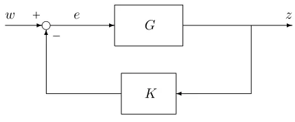
In this section we discuss a 1DOF mass-spring-damper system with mass m, spring stiffness k and damping co-efficient c. The values can be in any consistent system of units, for example, in SI units,min kilograms,kin newtons per meter, and c in newton-seconds per meter or kilograms per second. The system is of second order, since it has a mass which can contain both kinetic and potential energy. The forceF is considered as inputu, and the displacement pof the mass from the equilibrium position is considered as outputy of this system. By Hooke’s law, the force exerted by the spring is

Fs=−kp.

Let v be the velocity of the mass, then the damping force Fd is expressed as

Fd=−cv=−cdp

dt =−cp˙

due to d’Alembert’s principle. Using Newton’s second law, we have

F+Fs+Fd=m

d2_p dt2 =mp,¨ which gives

mp¨+cp˙+kp=u.

A possible selection of state variables is the displacement p and the velocityv. The linear model of the mass-spring-damper is then described by

G: (

˙

x=Ax+Bu y=Cx

where

A=

0 1

−k

m −

c m

, B=

0

1

m

andC=1 0.

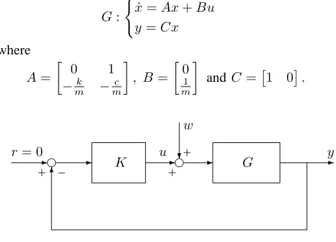
r= 0

-e

+ –

- _K u-_e

+

?

w

+

-G -y

[image:4.595.49.293.400.576.2]

6

Fig. 2. The structure of mass-damper-spring control system

The design objective for the mass-spring-damper system with a disturbance is to find an output feedback control law u=Ky which stabilizes the closed-loop system while minimizing worst-case energy of outputz= [y u]⊤ _{in order} to avoid the disturbance input w to affect the system. In realistic systems, the physical parameters k and c are not known exactly but can be enclosed in intervals. Assuming the controller is parameterized asK(κ), takingxto regroup

the tunable parametersk, candκ, and denoting byTw→z(x) the closed-loop performance channel w → z, this leads to the optimization problem

minimize kTw→z(x)k subject to x= (k, c, κ)∈Rn,

K=K(κ)assures closed-loop stability, kandc are in some intervals

(7)

where choices ofk · k include the H∞-normk · k∞ or the Hankel normk · kH.

VI. CLARKE SUBDIFFERENTIALS OF THEHANKEL NORM

In order to apply nonlinear and non-smooth optimization techniques to programs of the form (5), (6) and (7) it is necessary to provide derivative information of the objective function

f(x) =kG(x)k2

H =λ1(X(x)Y(x)),

whereX(x)andY(x)are the controllability and observabil-ity Gramians. In the discrete-time case,X(x)andY(x)can be obtained from the Lyapunov equations

A(x)XA⊤_{(x)−X+B(x)B}⊤_{(x) = 0, (8)} A⊤(x)Y A(x)−Y +C⊤(x)C(x) = 0. (9)

Remark that despite the symmetry ofX andY the product XY needs not be symmetric, but stability ofA(x)guarantees X≻0,Y ≻0in (8), (9), so that we can write

λ1(XY) =λ1(X12Y X21) =λ1(Y12XY 12),

which brings us back in the realm of eigenvalue theory of symmetric matrices.

Recalling the definition of the spectral radius of a matrix ρ(M) = max{|λ|:λeigenvalue ofM},

we can address programs (5) and (6) in the following program

minimize f(x) :=kG(x)k2

H

subject to c(x) :=ρ(A(x))−1 +ε60 (10)

for some fixed smallε > 0. Notice that f =k · k2

H◦G(·)

is a composite function of a semi-norm and a smooth mappingx7→G(x), which implies that it is lower-C2, and

therefore also lower-C1_{in the sense of [16, Definition 10.29].} Theoretical properties of the spectral radiusc(x), used in the constraint, have been studied in [3]. We also haveX(x)≻0

andY(x)≻ 0 on the feasible set C ={x :c(x)6 0}, so

thatf is well-defined and locally Lipschitz onC.

Let M_n,m be the space of n×m matrices, equipped with the corresponding scalar producthX, Yi= Tr(X⊤_Y), whereX⊤ _{andTr(X)are respectively the transpose and the} trace of matrix X. We denote by B_m the set of m×m symmetric positive semidefinite matrices with trace 1. Set Z :=X12Y X12 and pick Q to be a matrix whose columns

form an orthonormal basis of theν-dimensional eigenspace associated with λ1(Z). By [13, Theorem 3], the Clarke subdifferential of f at x consists of all subgradientsgU of

the form

gU = (Tr(Z1(x)⊤QU Q⊤), . . . ,Tr(Zn(x)⊤QU Q⊤))⊤,

where U ∈ B_ν, and where Mi(x) := ∂M(x)

∂xi , i = 1, . . . , n for any matrixM(x).We next have

Zi(x) =χi(x)Y X12 +X 1 2Yi(x)X

1

2 +X

1

2Y χi(x), (11)

whereχi(x) :=∂X

1 2(x)

∂xi . It follows from(8)and(9)that A(x)Xi(x)A⊤(x)−Xi(x) =−Ai(x)XA⊤(x)

−A(x)X[Ai(x)]⊤_−Bi(x)B⊤_{(x)−B(x)[Bi(x)]}⊤_{, (12)} A⊤_{(x)Yi(x)A(x)−Yi(x) =−[Ai(x)]}⊤_{Y A(x)}

Since X12X 1

2 =X,

X12χi(x) +χi(x)X12 =Xi(x). ₍₁₄₎

Altogether, we obtain Algorithm 2 to compute elements of the subdifferential off(x).

Algorithm 2

_.

Computing subgradients.

Input: x∈Rn. Output:g∈∂f(x).

1: Compute Ai(x) = ∂A(x)

∂xi , Bi(x) =

∂B(x)

∂xi , Ci(x) = ∂C(x)

∂xi , i = 1, . . . , n and X, Y solutions of (8), (9), respectively.

2: ComputeX12 andZ=X12Y X12.

3: Fori= 1, . . . , ncomputeXi(x)andYi(x)solutions of (12) and (13), respectively.

4: For i = 1, . . . , n compute χi(x) solution of (14) and Zi(x) using (11).

5: Determine a matrixQwhose columns form an orthonor-mal basis of the ν-dimensional eigenspace associated withλ1(Z).

6: PickU ∈B_ν, and return

(Tr(Z1(x)⊤_{QU Q}⊤_{), . . . ,Tr(Zn(x)}⊤_{QU Q}⊤₎₎⊤_,

a subgradient off atx.

Remark 1: In the continuous-time case, the Gramians

X(x)and Y(x)can be obtained from the continuous Lya-punov equations

A(x)X+XA⊤_{(x) +B(x)B}⊤_{(x) = 0, (15)} A⊤_{(x)Y +Y A(x) +C}⊤_{(x)C(x) = 0, (16)}

Therefore,Xi(x)andYi(x)are solutions respectively of the following equations

A(x)Xi(x) +Xi(x)A⊤_{(x) =−Ai(x)X−X[Ai(x)]}⊤ −Bi(x)B⊤(x)−B(x)[Bi(x)]⊤, (17) A⊤_{(x)Yi(x) +Yi(x)A(x) =−[Ai(x)]}⊤_{Y −Y Ai(x)}

−[Ci(x)]⊤_C(x)−C⊤_(x)C

i(x). (18)

In addition, let us note that for this case, the stability constraint in program (10) is c(x) = α(A(x)) +ε 6 0, whereα(·)denotes the spectral abscissa of a square matrix, i.e., the maximum of the real parts of its eigenvalues.

We now introduce a smooth relaxation of Hankel norm. It is based on a result established by Y. Nesterov in [9], which gives a fine analysis of the convex bundle method in situations where the objectivef(x)has the specific structure of a max-function, including the case of a convex maximum eigenvalue function. These findings indicate that for a given precision, such programs may be solved with lower algo-rithmic complexity using smooth relaxations. While these results are a priori limited to the convex case, it may be interesting to apply this idea as a heuristic in the non-convex situation. More precisely, we can try to solve problem (10), (2) by replacing the functionf(x) =λ1(Z(x))by its smooth approximation

fµ(x) :=µln nx

X

i=1

eλi(Z(x))/µ

!

, (19)

whereµ >0is a tolerance parameter,nxthe order of matrix

Z, and whereλi denotes the ith eigenvalue of a symmetric

or Hermitian matrix. Then

∇fµ(Z) = nx

X

i=1

eλi(Z)/µ

!−1 _nx X

i=1

eλi(Z)/µ_qi(Z)qi(Z)⊤_,

with qi(Z) the ith column of the orthogonal matrix Q(Z) from the eigendecomposition of symmetric matrix Z= Q(Z)D(Z)Q(Z)⊤_{. This yields}

∇fµ(x) =

(Tr(Z1(x)⊤∇fµ(Z)), . . . ,Tr(Zn(x)⊤∇fµ(Z)))⊤.

Let us note that

f(x)6fµ(x)6f(x) +µlnnx.

Therefore, to find anǫ-solution of problem (2), we have to find an ₂ǫ-solution of the smooth problem

minimize fµ(x)

subject to c(x)60

Ax6b

(20)

withµ= _{2 ln}ǫ_nx. This smoothed problem can be solved using standard NLP software. We have initialized the non-smooth algorithm 1 with the solution of problem (20).

VII. NUMERICAL EXPERIMENTS A. Steady Flow in a Graph

We give an illustration of programs (5) and (6). Let V_{stay = {1,2, . . . , nx},} V_{in = {1,2, . . . , m} and} V_{out = {1,2, . . . , p}. Taking x to regroup the unknown} tunable parametersajj′, bij and settingA(x) = [ajj′]⊤_nx×nx, B(x) = [bij]⊤

m×nx, C = [c1, . . . , cnx], where ajj′ = 0 if

(j, j′_{)6∈A, b}

ij = 0 if (i, j) 6∈A, we have a discrete LTI

system

G(x) : (

x(t+ 1) =A(x)x(t) +B(x)w(t)

z(t) =Cx(t).

Note that the linear constraint conditions in (5) as well as (6) can be transferred to the form

(

Aeqx=beq,

x>0.

We now take the graph G _{= (}V_,A_{) with nx = 36,} m = 2 and p = 2 as in Figure 3. Let z(t) be the total number of individuals inside the fairground with doubled weights at 6 nodes in the center that form a hexagon as compared to the other nodes. We start with the case without controller and initialize at the uniform distribution

x1, wheref(x1) = 528.7672andkG(x1)kH = 22.9949. In

order to save time, we use the minimizer of the relaxation fµ(x) in (19) with initial x1 to initialize the non-smooth

algorithm 1. Our algorithm then returns the optimalx† with

f(x†_{) = 16.5817, meaningkG(x}†_)k

H= 4.0721.

In the case with controllerK=K(κ),κ= [κ1 . . . κm]⊤_, as shown in Figure 1, we have

Tw→z(x, κ) :

(

x(t+ 1) =A(x)x(t) +B(x)e(t)

[image:6.595.131.463.49.148.2]

i1 o1 1 2 3 4 5 6 7 8 9 10 11 12 13 14 15 16 17 18 19 20 21 22 23 24 25 26 27 28 29 30 31 32 33 34 35 36 i2 o2

Fig. 3. Model of the fairground.

Heree(t) =w(t)−Kz(t) =w(t)−KCx(t), which gives

Tw→z(x, κ) =

A(x)−B(x)K(κ)C B(x)

C 0

.

Initializing at (x, κ) = (x1_{,0) with remarking that} Tw→z(x,0) =G(x)and proceeding as in the previous case, we obtain the optimal (x∗_{, κ}∗_{) with f(x}∗_{, κ}∗_{) = 2.0001,} meaning kTw→z(x∗, κ∗)kH = 1.4142. Step responses and

ringing effects in unit step and white noise responses trun-cated atT = 30for the three systemsG(x1_{) =T}

w→z(x1,0), G(x†_{) and T}

w→z(x∗, κ∗) are compared in Figure 4 and Figure 5.

0 20 40 60 80 100 120 140 0 5 10 15 20 25 30 35 From: In(1)

[image:6.595.307.543.185.386.2]

0 20 40 60 80 100 120 140 From: In(2) Step Response Time (seconds) Amplitude initial without controller with controller

Fig. 4. Experiment 1. Step responses of three systemsG(x1)(dotted), G(x†)(dashed) andTw→z(x∗, κ∗)(solid).

B. Robust Control of a Mass-Spring-Damper System

Here we apply Algorithm 1 to solve problem (7), where the mass-spring-damper plant with a disturbance is given by

P :  xz˙

y 

=

 

A B1 B

C1 0 D12

C 0 0

   wx

u  , with A= 0 1

−_mk −_mc

, B1=B= 0 1 m C1= 1 0 0 0

, D12=

0 1

andC=1 0.

0 20 40 60 80

−5 0 5 10 15 20 25

Unit step signal From: In(1)

Time (seconds)

0 20 40 60 80

−5 0 5 10 15 20 25

Unit step signal From: In(2)

Time (seconds)

0 20 40 60 80

−5 0 5 10 15

White noise signal From: In(1)

Time (seconds)

0 20 40 60 80

−5 0 5 10 15

White noise signal From: In(2)

Time (seconds) initial without controller with controller

Fig. 5. Experiment 1. Ringing effects of three systemsG(x1)(dotted),

G(x†)(dashed) andTw→z(_x∗, κ∗)(solid). Input: Unit step signal (top)

and white noise signal (bottom).

The controllerKis chosen of order 2, namely

K(κ) =κ1s

2_+κ2s+κ3

s2_+κ4s+κ5

=  

−κ4 κ5 1

1 0 0

κ2−κ1κ4 κ3−κ1κ5 κ1  :=

AK BK

CK DK

.

Then, the closed-loop transfer function of the performance channel channelw→z has the state-space representation

Tw→z(x) :

_˙ ξ z =

A(x) B(x)

C(x) 0

ξ w

,

whereξ= [x xK]⊤,xK the state ofK, and where

A(x) =

A+BDKC BCK

BKC AK

,

B(x) =

B1+BDKD21

BKD21

,

C(x) =C1+D12DKC D12CK.

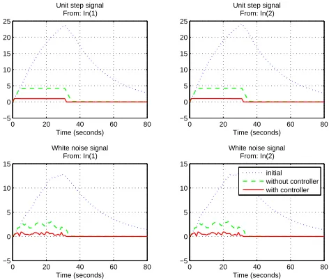
Assume that massm= 4, and spring stiffnesskand damping coefficient c belong to the intervals [4,12] and [0.5,1.5], respectively. Using the Matlab functionhinfstructbased on [1], we optimizedH∞-norm and obtainedk= 12, c= 1 and

K∞=

[image:6.595.52.288.360.553.2]

In the Hankel norm synthesis case, our Algorithm 1 returned k= 12, c= 1.5 and

KH =

[image:7.595.51.289.161.351.2]

−6.1975s2_{−2.1828s−4.2523} s2_{+ 19.3261s+ 3.9198} .

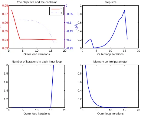
Figure 6 compares step responses and white noise responses in two synthesis cases. Bearing of the algorithm is shown in Figure 7.

0 10 20 30

0 0.05 0.1 0.15 0.2

Step response

Displacement

0 10 20 30

−0.1 −0.05 0 0.05 0.1 0.15

Velocity

Time (seconds)

0 10 20 30

−0.2 −0.1 0 0.1 0.2

White noise response

0 10 20 30

−0.4 −0.3 −0.2 −0.1 0 0.1 0.2 0.3

Time (seconds) H_∞−synthesis Hankel norm synthesis

Fig. 6. Experiment 2. Step responses (left) and white noise responses (right) in two synthesis cases.

0 5 10 15 20

0.03 0.04 0.05 0.06 0.07 0.08

The objective and the contraint

Outer loop iterations

f(x

j)

0 5 10 15 20−0.25

−0.2 −0.15 −0.1 −0.05 0

c(x

j) f c

0 5 10 15 20

0 0.2 0.4 0.6 0.8 1

Step size

Outer loop iterations

0 5 10 15 20

1 1.2 1.4 1.6 1.8 2

Number of iterations in each inner loop

Outer loop iterations

0 5 10 15 20

0 0.2 0.4 0.6 0.8 1

Memory control parameter

[image:7.595.56.289.405.597.2]

Outer loop iterations

Fig. 7. Experiment 2. Bearing of the algorithm.

VIII. CONCLUSION

We have shown that it is possible to optimize plant and controller simultaneously if the idea of a structured control law introduced in [1] is applied. Our approach was illustrated for Hankel norm synthesis as well as forH∞-synthesis, and for a continuous and a discrete system. Due to inherent non-smoothness of the cost functions, non-smooth optimization was applied, and in particular, a non-convex bundle method was presented. For eigenvalue optimization, as required for Hankel norm synthesis, a relaxation developed by Nesterov for the convex case was successfully used as a heuristic in the non-convex case to initialize the bundle method.

REFERENCES

[1] P. Apkarian and D. Noll, ”NonsmoothH∞ synthesis,” IEEE Trans.

Automat. Control, vol. 51, no. 1, pp. 71-86, 2006.

[2] P. Apkarian and D. Noll, ”Nonsmooth optimization for multidiskH∞ synthesis,” Eur. J. Control, vol. 12, no. 3, pp. 229-244, 2006. [3] J. V. Burke and M. L. Overton, ”Differential properties of the spectral

abscissa and the spectral radius for analytic matrix-valued mappings,” Nonlinear Anal., vol. 23, no. 4, pp. 467-488, 1994.

[4] F. H. Clarke, ”Generalized gradients of Lipschitz functionals,” Adv. in Math., vol. 40, no. 1, pp. 52-67, 1981.

[5] F. H. Clarke, Optimization and Nonsmooth Analysis, John Wiley & Sons, Inc., New York, 1983.

[6] N. M. Dao and D. Noll, ”Minimizing the memory of a system,” in Proceedings of the 9th Asian Control Conference, Istanbul, 2013. [7] M. Gabarrou, D. Alazard and D. Noll, ”Design of a flight control

architecture using a non-convex bundle method,” Math. Control Signals Systems, vol. 25, no. 2, pp. 257-290, 2013.

[8] K. Glover, ”All optimal Hankel-norm approximations of linear multi-variable systems and theirL∞_{-error bounds,” Int. J. Control, vol. 39,} no. 6, pp. 1115-1193, 1984.

[9] Y. Nesterov, ”Smoothing technique and its applications in semidefinite optimization,” Math. Program., Ser. A, vol. 110, no. 2, pp. 245-259, 2007.

[10] D. Noll, ”Cutting plane oracles to minimize non-smooth non-convex functions,” Set-Valued Var. Anal., vol. 18, no. 3-4, pp. 531-568, 2010. [11] D. Noll, ”Convergence of non-smooth descent methods using the

Kurdyka-Łojasiewicz inequality,” J. Optim. Theory Appl., to appear. [12] D. Noll, O. Prot and A. Rondepierre, ”A proximity control algorithm

to minimize nonsmooth and nonconvex functions,” Pac. J. Optim., vol. 4, no. 3, pp. 571-604, 2008.

[13] M. L. Overton, ”Large-scale optimization of eigenvalues,” SIAM J. Optim., vol. 2, no. 1, pp. 88-120, 1992.

[14] A. M. Ostrowski, Solutions of Equations in Euclidean and Banach Spaces, Pure and Applied Mathematics, Vol. 9. Academic Press, New York-London, 1973.

[15] E. Polak, Optimization: Algorithms and Consistent Approximations, Applied Mathematical Sciences, 124. Springer-Verlag, New York, 1997. [16] R. T. Rockafellar and R. J.-B. Wets, Variational Analysis,