Abstract—In this work, the impact of economic cycle on a stock price was investigated via the excess demand and supply. The economic cycle was treated as external influence which determines how the investor takes his decision on trading. The external influence was prototypically prescribed as a sinusoidal function, where excess demand and supply were calculated using Ising Hamiltonian and the mean-field technique in Econophysics. The fourth order Runge Kutta was used to extract the investors’ demand/supply as well as the stock price as a function of time. From the results, it is found that the external influence characteristic and market temperature have significant effect on the price changes, resulting in different characteristic of price return distribution. Specifically, lower external influence period broadens the return distribution, whereas larger market temperature results in an opposite way. This work therefore serves as an elementary base of modeling stock price when considering the external influence as dynamically changeable periodic parameters, and suggest how price and price return would react to this active behavior of the economic cycle.
Index Terms—Economic cycle, Econophysics, Ising model, Mean-field, Stock market
I. INTRODUCTION
HE stock market is an important system for companies to raise money, which supports both economic and financial development of the country [1]. It is where a large number of investors interact with one another as well as external influences/information to determine the best price for a given stock [2]. Typically, status of the stock market can indicate overall economic conditions as the stock market and the economic cycle are mutually dependent. This is since investors tend to leave the market at economic contraction and return to the market during economic recovery leading to periodic cycle of stock price variation. Generally, due to interaction among investors, even there is not a solid bad news but if there is a panic sell, an individual investor may lose confident to hold his stock and sell to stop loss. Nevertheless, when there is panic buy, the same investor may be inspired to buy unless he could be fallen behind. In addition, the investors’ decision is also shaped by external influences. For instance, if there is a
Manuscript received July 26, 2016; revised August 16, 2016.
Y. Laosiritaworn*, C. Supatutkul and S. Pramchuare are with the Department of Physics and Materials Science, Faculty of Science, Chiang Mai University Chiang Mai, Thailand (*corresponding author’s e-mail address: [email protected]).
succession of bad economic news, this tends to discourage people from spending/investing leading to economic recession. However, when the economy recovers, this will encourage consumers to spend and invest more, which leads to economic growth. External influence is then an important factor to cause the economic cycle.
The economic cycle is a natural fluctuation of the economy between periods of economic growth and economic recession. Factors such as gross domestic product (GDP), interest rates, levels of employment, consumer spending, and government’s fiscal policy can help to determine the current stage of the economic cycle. This economic cycle also causes the periodic changing of the price and return of the stock market [3], introducing “bull” and “bear” periods. It is believed that recognizing “bull” and “bear” cycles is a key to make money from stock market. Also, the understanding of economic cycle may help realizing when bubble and crash situations is about to happen. Note that when the bubble bursts, there will be a significant drop in the market value, which yields great negative impacts on the economy. Therefore, it is essential to possess knowledge that can comprehend the status of the stock market to predict when these undesired situations are about to occur. Recently, one aspect that can deal with these situations is econophysics.
Econophysics combines both economics and physics to seek for fundamental underlying about market dynamics, investor behaviors, and wealth distribution in the community using relationship among investors and economical sources [4]. Concepts of classical mechanics, thermodynamic, statistical mechanics, etc., are usually used to solve problems in Economics [4]-[5]. There were many recent studies proposed on the stock price using econophysics techniques. For instance, the use of continuous-time random walk to relate the waiting-times and returns in high-frequency financial data [6], or the use of Monte Carlo technique and Fokker-Planck equation to solve for collective dynamics of stock prices [7]. There were also works related to establishing volume-price relationship of the stocks and predict the characteristic of the market via distribution of the return (e.g. see reviews given in [8]-[9]). However, most previous works considered effect of external influences on investors as well-defined static values, e.g. see [10]. Nevertheless, in real system, external influences usually comprehend economic cycle which should be considered as periodic functions. Therefore, this work aims
Computational Econophysics Simulation of
Stock Price Variation Influenced by
Sinusoidal-like Economic Cycle
Yongyut Laosiritaworn*, Chumpol Supatutkul and Sittichain Pramchu
to investigate the effect of the economic cycle, treated as external influence, on buying/selling decision of the investors. This external influence was prototypically assumed as a simple sinusoidal function, and the decision of buying and selling was determined by solving the Ising spin Hamiltonian under the framework of mean-field theory in statistical physics.
II. THEORY AND METHODOLOGY
A. Ising Spin Hamiltonian and Econophysics
An important model in econophysics is the agent-based model. This model was devised from statistical physics, where the usual considered system is a magnetic system. In the simplest one, the system contains magnetic spins, that each can have only 2 possible discrete states, called Ising spin. These different states can be applied to economic by refereeing to states of an individual investor in stock market, e.g. “+1” for intention to “buy or ask” and “-1” for intention to “sell or bid”. The average of the all spin states, called magnetization, can be related to average intention to buy or to sell the stock each individual holds. For instance, if the magnetization is negative, the investor may want to sell his stock and the price of the stock may drop. However, if the magnetization is positive, the investor may want to buy and the price may increase. Nevertheless, for zero magnetization, the current price is hold due to demand-supply agreement.
In nature, all systems have least energies at ground state. Therefore, by adopting the Ising energy (or Hamiltonian H) into economics, the state of investors’ decision on buying and selling actions can be described by [5]
,
i j i
i j i
H J h
. (1)As is seen, the energy or the Hamiltonian H in (1) is the sum of 2 terms. The first term (
, i j
i j
J
) is due to the interactions among spins with a strength J. Here, the spini = 1 is the Ising spin (investor, agent) where +1 and -1
are for tendencies to buy and sell, respectively. The notation <i,j> considers only finite number of neighbor spins in the sum. This is the same in real stock market as the influence of buying or selling on an investor usually comes from individuals that have close relationship to that investor. Note that when all spins are equal to 1 or -1, H is minimized (most negative), which is the case for ground state in nature. In economics, this state can be referred to extreme conditions where all investors go for panic buying or selling. The second term (h
ii ) in (1) is the external influence, which could come from the company’s financial situation, market trends, economic cycle, etc. The positive h refers to the period of economic prosperity, where people have purchasing power leading to an intention to buy. Meanwhile, the negative h is for economic recession, where the purchasing power declines inducing the excess
minimize H.
In statistical physic, the solution to (1) can be defined from the magnetization
1/
ii
m N
, where N is the total number of members in the system. Typically, mdepends on temperature T. At high temperatures, the energy is abundant so each spin has sufficient energy to break the bond specified by the interaction strength J. Therefore, all spins arrange in a random fashion and m
0. This is when demand and supply equivalently match in stock market. Whenever there is a demand, there is always a supply to close the deal, or vice versa, without taking any limit orders. This reflects high liquidity level of that stock in the market. Nevertheless, for low temperatures such as T
0, the system arrives in its extreme states either overloading demand (m +1) or supply (m +1) states, causing the price to dramatically change subsequently. Also, not only T but also h that m depends on. If h is a constant (a static condition), the system will arrive at an equilibrium state where m is also a constant. However, if h
is changeable with time t (to mimic real economic cycle), m
will change with time t too, i.e. m = m(t). Further, according to this dynamic behavior, once the system arrives in its steady state, the relationship between m(t) and h(t) will form a so called hysteresis loop, which the hysteresis shapes indicate how investors’ decision depends on the influences.
B. Mean Field Theory
To solve (1) for m(t) is generally very complicated due to the large number of degree of freedom, arisen from number of members in the system. However, one could simplify this many body spin-spin interaction problems into a single body problem where each individual spin interacts with only an effective influence acting on itself via a mean-field framework. In brief details, by considering the Hamiltonian in (1), the dynamic of magnetization m under the influence of the time-varying external influence h(t) can be given by [11]-[12]
( )
( ) tanh
dm t
m t E
dt
, (2)
where τ is the time interval of each spin changing its state. In (2), the parameter ( ) ( )
B
zJm t h t E
k T
describes the
conclusive effect from spin-spin interaction, the external influences, and the temperature T. Here, z is the number of neighboring spins that each individual spin interacts with,
β =1/kBT, and kB is the Boltzmann’s constant. Then, to
incorporate with the economic cycle, a simple case where the external influence takes the simple sinusoidal harmonic form, i.e.h t
h0sin 2
t P/
where h0 and P are the external influence amplitude and period respectively was considered. For conveniences, = 1 was set as unit of time and by introducing reduced parameters T k T zJB / and/
0sin 2
/
( )
( ) tanh m t h t P
dm t
m t
dt T
, (3)
which can be solved using the fourth order Runge-Kutta method [14]. Next, the data (h(t), m(t)) was plotted to form hysteresis loops which provide information how decision of the investor varies with external influence.
C. Stock Price and Magnetization Relationship
In a stock market, there generally consists of 2 types of the investors, i.e. fundamental and interacting investor. The fundamentalist is assumed to know the fundamental (reasonable) price Pfund(t) of the stock. If the current price
P(t) is less than Pfund(t), the fundamental investor will be
likely to buy the stock, and sell otherwise. The amount of selling/buying orders issued by a fundamentalist takes a non-linear relationship with the differences between the current and fundamental prices as [15]
ln
ln
fund fund fund fund
x t a N p t p t , (4)
where xfund is the amount of fundamental orders, Nfundis the
number of fundamental investors, and afund is a constant.
Apart from fundamental orders, the interacting orders are also important to determine where demand meets supply. The interacting orders are supplied by interacting investors, i.e. the spins in (1), and the interacting investors’ excess demand for the stock can be estimated from [15]
inter inter inter
x t a N m t , (5)
where xinter is the amount of the interacting orders, Ninteris
the number of interacting investors, and ainter is another
constant. As a result, the market clearing price can be defined from the demand and supply being in balance, i.e.
0fund inter
x t x t or
lnp t lnpfund t km t ; p t pfund t ekm t , (6)
where inter inter 0
fund fund
a N
k
a N
. Considering the price equation in (6), it is possible to classify the market in several situations. For instance, for m(t) = 0, the market price p(t) stay at the fundamental price pfund(t). On the other hand, for
m(t) > 0, there are excess demand which pushes p(t) to surpass the pfund(t), resulting in a bull market. Nevertheless,
for m(t) < 0, the price p(t) drops below the pfund(t), bringing
about bear period in the market.
It is also of interest to investigate the performance of the proposed model via the return parameter
lnp t
lnp t
r t m t m t
k
(7)
where is the time lag, and the fundamental price is assumed unchanged during the considered economic cycle, i.e. pfund(t) = pfund(0). Then, with histogram analysis
between N r
and r, the relationship in the form [8]
1 N r r (8)
is usually found, where 1+ is the exponent to the scaling which is the characteristic of an individual stock market.
III. RESULTANDDISCUSSION
In order to obtain magnetization as a function of time, the mean field equation in (3) was solved via the fourth order Runge Kutta method [14] with initial m(0) = 1.0 and time step t = P/NP where P is the period of the external
influence, and NP is number of data point measured in one
cycle. This work considered {P,NP} = {1000,600} and
{100,300}. Next, the period average magnetization
0
P
Q
m t dt Pwas used to judge how many cycles todiscard for steady state, i.e. when Q is no longer time dependent [16]. The considered external influence and temperature parameters chosen in this work were h0= 0.5 and 2.0 J/z, P = 100 and 1000 , and T = 0.5 and 2.0 J/zkB.
These parameters were chosen to ensure the symmetric behavior of the (m,h) hysteresis loop [13] which is unbiased situation in the economic cycle. It was found that 500 loops (cycles) were enough to reach the steady state. After that,
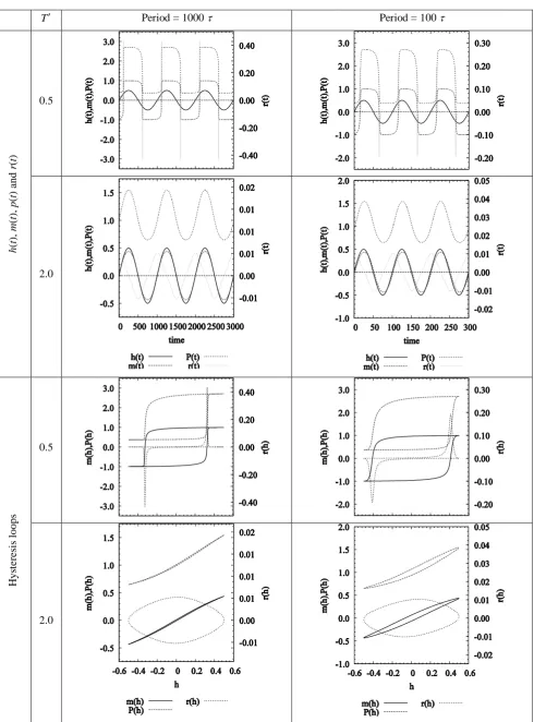
h(t), m(t), p(t) (with k fixed at 1) and r(t) for = t were recorded/calculated as a function of t, e.g. see Fig. 1.
As seen in Fig. 1, the external influence and temperature both have significant on the m(t), p(t) and r(t). For instance, with increasing T, the hysteresis loops become slimmer suggesting lower phase-lag between h and other corresponding m and p signals. This is expected as when the market is with high liquidity, investors trade very often where the price will either increase or decrease depending on there is good news or bad news (sign of the h). In addition, with increasing period P, the loops are also broader. This is as the larger period of the news cycles, the more time an investor has in responding to the economic situation. Hence, both m and P have more chances to promptly respond to h and hence yielding slimmer (h(t),m(t)) and (h(t),p(t)) loops.
T Period = 1000 Period = 100
h
(
t
),
m
(
t
),
p
(
t
)
a
nd
r
(
t
)
0.5
2.0
H
ys
te
re
si
s
loops
0.5
[image:4.595.51.542.56.718.2]2.0
Figure 2. Histrogram N(r) of the return r specifying the price return distribution for the external influcne with peiod = {100 , 1000 ) and amplitude h0= 0.50 for tempearutre (a) T = 0.5 and (b) T = 2.0.
IV. CONCLUSION
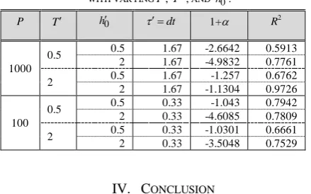
This work considered the effect of economic cycle (via external influence cycle) in a simple sinusoidal form to investigate excess demand/supply in extracting the stock price variation as a function of external influences and time. The relationship among the investors’ decision on buying/selling, the stock price, and the price return were investigated and compared with the value of the external influence in both time and influence domain. The hysteresis loop of the influence and the corresponding parameters were drawn and discussed. Then, the price return distribution was also analyzed to extract the exponent to the distribution scaling. However, due to time-lag limited in this work, the R2 prevents quantitatively comparison with real market. However, the exponent values still give sensible results how the market reacts when changing the external influence parameter and temperature, giving a basis ground-base for further detailed analysis of the time-lag dependence on price-distribution in the forthcoming studies.
REFERENCES
[1] R. Levine and S. Zervos, “Stock markets, banks, and eonomic growth,” Am. Econ. Rev., vol. 88, pp. 537-558, June 1998.
[2] Y. Yu, W. Duan, and Q. Cao, “The impact of social and conventional media on firm equity value: A sentiment analysis approach,” Decis. Support. Syst., vol. 55, pp. 919-926, November 2013.
[3] H. Schaller and S. Van Norden, “Regime switching in stock market returns,” Appl. Finan. Econ., vol. 7, pp. 177-191, October 2010. [4] R.N. Mantegna, H.E. Stanley, An Introduction to Econophysics:
Correlations and Complexity in Finance. Cambridge: Cambridge University press, 2000.
[5] J. Voit, The Statistical Mechanics of Financial Markets, 3rd ed. Berlin: Springer, 2005.
[6] M. Raberto, E. Scalas, F. Mainardi, “Waiting-times and returns in high-frequency financial data: an empirical study,” Physica A, vol 314, pp. 749-755, November 2002.
[7] T. D. Frank, “Exact solutions and monte carlo simulations of self-consistent langevin equations: A case study for the collective dynamics of stock prices,” Int. J. Mod. Phys. B, vol. 2, pp. 1099-1112, March 2007.
[8] A. Chakraborti, I. M. Toke, M. Patriarca, and F. Abergel, “Econophysics review: I. Empirical facts,” Quant. Financ., vol. 11, pp. 991-1012, June 2011.
[9] A. Chakraborti, I. M. Toke, M. Patriarca, and F. Abergel, “Econophysics review: II. Agent-based models,” Quant. Financ., vol. 11, pp. 1013-1041, June 2011.
[10] A. Thongon , S. Sriboonchitta, and Y. Laosiritaworn, “Affect of markets temperature on stock-price: Monte Carlo simulation on spin model,” AISC, vol. 251, pp. 445-453, 2014.
[11] M. Suzuki and R. Kubo, “Dynamics of the Ising model near the critical point. I,” J. Phys. Soc. Jpn., vol. 24, pp. 51-60, January 1968. [12] B.K. Chakrabarti and M. Acharyya, “Dynamic Transitions and
Hysteresis,” Rev. Mod. Phys., vol. 71, pp. 847-859, April 1999. [13] A. Punya, R. Yimnirun, P. Laoratanakul, and Y. Laosiritaworn,
“Frequency dependenceoftheIsing–hysteresisphase–diagram: Mean fieldanalysis,” Physica B, vol. 405, pp. 3482-3488, August 2010. [14] W.H. Press, B.P. Flannery, S.A. Teukolsky and W.T. Vetterling,
Numerical Recipes in C. Cambridge: Cambridge University Press, 1988.
[15] T. Kaizoji, S. Bornholdt, Y. Fujiwara, “Dynamics ofprice and trading volume in a spin model ofstock markets with heterogeneous agents,” Physica A, vol. 316, pp. 441- 452, December 2002.
[16] Y. Laosiritaworn, A. Punya, S. Ananta, R. Yimnirun, “Mean-Field Analysis of the Ising Hysteresis Relaxation Time,” Chiang Mai J. Sci., vol. 36, pp. 263-275, September 2009.
TABLEI
RESULTS OF THE POWER LAW FITTING INDICATING THE EXPONENT (1+) WITH VARYING P,T, AND h0.
P T h0 dt 1+ R2
1000
0.5 0.5 1.67 -2.6642 0.5913
2 1.67 -4.9832 0.7761
2 0.5 1.67 -1.257 0.6762
2 1.67 -1.1304 0.9726
100
0.5 0.5 0.33 -1.043 0.7942
2 0.33 -4.6085 0.7809
2 0.5 0.33 -1.0301 0.6661
[image:5.595.53.273.343.480.2]