Weather effects on human mobility : a study using multi channel sequence analysis

WEATHER EFFECTS ON HUMAN MOBILITY: AN ANALYSIS USING MULTI-CHANNEL

SEQUENCE ANALYSIS

Vanessa S. Brum-Bastos

_{, Jed A. Long}

_{, Urška Demšar}

1

_{School of Geography & Sustainable Development, University of St Andrews,}

Irvine Building, North Street, St Andrews, UK

5 

Email: {vdsbb*, jed.long, urska.demsar}@st-andrews.ac.uk

*Corresponding author

Abstract

Widespread availability of geospatial data on movement and context presents opportunities for

10 

applying new methods to investigate the interactions between humans and weather conditions.

Understanding the influence of weather on human behaviour is of interest for diverse applications,

such as urban planning and traffic engineering. The effect of weather on movement behaviour can be

explored through Context-Aware Movement Analysis (CAMA), which integrates movement geometry

with its context. More specifically, we use multi-channel sequence analysis (MCSA) to represent a

15 

person’s movement as a multi-dimensional sequence of states, describing either the type of

movement or the state of the environment throughout time. Similar movement patterns can then be

identified by comparing and aligning mobility sequences. In this paper we apply CAMA and MCSA to

explore weather effects on human movement patterns. Data from a GPS tracking study in a Scottish

town of Dunfermline are linked to weather data and converted into multi-channel sequences which are

20 

clustered into groups of similar behaviours under specific weather typologies. Our findings show that

the CAMA + MCSA method can successfully identify the response of commuters to variations in

environmental conditions. We also discuss our findings on how travel modes and time spent at

different places are affected by meteorological conditions, mainly wind, but also rainfall, daylight

duration, temperature, comfort and relative humidity.

25 

Keywords:

context-aware movement analysis, context-aware similarity, human mobility, human

movement, multi-channel sequence analysis, context.

1. Introduction

The spread of geolocated smartphones and the decreasing price of GPS devices have contributed

towards the production of large amounts of data on human movement of unprecedented

spatio-30 

temporal quality (Meekan et al., 2017). New human mobility studies attempt to link such movement

data with contextual information (such as points of interest) to gather insights into, for example,

commuting behaviour (Beecham, Wood, & Bowerman, 2014; Gong, Chen, Bialostozky, & Lawson,

2012), tourist behaviour (Meijles, de Bakker, Groote, & Barske, 2014; Versichele, Neutens,

Delafontaine, & Van de Weghe, 2012), or retail choice decisions and human activities (Si

ł

a-Nowicka

35 

Manuscript accepted to 

Computers, Environment and Urban Systems

, May 2018 

tourism (de Freitas, 2003), health (Tucker & Gilliland, 2007), psychology (Nerlich & Jaspal, 2014) and

40 

epidemiology (Horowitz, 2002).

Specific weather conditions often trigger changes in human behaviour, for example, higher

temperatures increase aggressiveness (Anderson, 2001; Carlsmith & Anderson, 1979) and lower

temperatures contribute to irritability and combativeness (Schneider, Lesko, & Garret, 1980; Worfolk,

1997). Different components of weather have different magnitudes of importance, for example, air

45 

temperature, direct solar radiation and wind speed have a more significant influence on human

behaviour than humidity (de Montigny, Ling, & Zacharias, 2012). However, it is challenging to

understand how weather influences human behaviour because the responses are partially a result of

individual preferences (de Freitas, 2015). Some individuals are more responsive to the thermal

component of weather, i.e. the combined effects of air temperature, humidity and solar radiation, while

50 

some are more receptive to physical components like rain, and others are more greatly affected by

the aesthetic components, such as cloud coverage and sunshine. Yet, most individuals do respond to

the combination of all three of these components (de Freitas, 1990).

Traditionally, these interactions have been explored through questionnaires and multidimensional

scaling methods within the field of human biometeorology (Cabanac, 1971; de Freitas, 1990; Manu,

55 

Shukla, Rawal, Thomas, & de Dear, 2016). With the increased availability of tracking and

environmental data we however propose that the effect of weather on movement behaviour can be

explored through Context-Aware Movement Analysis (CAMA), which integrates movement geometry

with its context, i.e. with the surrounding biological and environmental conditions that might be

affecting movement (Andrienko, Andrienko, & Heurich, 2011; Demsar et al., 2015; Dodge et al.,

60 

2013). More specifically we use multi-channel sequence analysis (MCSA) to represent a person’s

movement as a sequence of states, describing either the type of movement or the state of the

environment throughout time. Similar movement patterns can then be identified (termed context

aware similarity analysis) by comparing and aligning mobility sequences.

Similarity analysis is one of the most common tasks in movement analytics and consists of using

65 

geometry or physical attributes; geometrical similarity solely relies on measures of spatial and

70 

temporal distances, and physical similarity relies on movement attributes such as speed, turning

angle, acceleration and direction (Demsar et al., 2015). Context-aware similarity is based on multiple

attributes (Andrienko et al., 2011; Buchin, Dodge, & Speckmann, 2014; Demsar et al., 2015; Sharif &

Alesheikh, 2017b) describing the conditions within which the movement took place.

Context-awareness is a recent trend (Sharif & Alesheikh, 2017a), as a result there are few

context-75 

aware methods for assessing similarity between trajectories. Sharif & Alesheikh (2017b) generalized

the dynamic time warping (DTW) to develop a context-based dynamic time warping (CDTW) method,

which matches trajectories with contextual similarity even if they are not concurrent. This method is

highly dependent on arbitrary weights for the contextual variables, restricted to numeric context and

disregards changes of context between two points in time. i.e., same contexts are considered similar

80 

even when they are not concurrent. De Groeve et al. (2016) uses single channel sequence

alignments and Hamming Distance to understand the temporal variation of habitat use by roe deer;

the similarity is measured by the cost to transform a sequence of habitat use into another. This

method is able to handle only one contextual variable at time, therefore it is not able to handle the

interactive effect of multiple contextual variables on movement. Buchin et al. (2014) modified existing

85 

similarity measures to make them context-aware, more specifically they defined the distance between

two points as the sum of their contextual and spatial distances. The transition costs between contexts

are defined by the user and the method is restricted to contextual data in the form of polygonal

divisions.

In this paper we propose to use multi-channel sequence analysis (MCSA) to perform context-aware

90 

similarity analysis (CASA) and cluster trajectories into groups of similar behaviour. MCSA is a new

analysis tool for movement data where contextual information can now be readily combined with

detailed tracking datasets. The main advantage of this approach is that it also is possible to consider

as many channels (contextual variables) as desired at once. It is common in movement research to

simultaneously consider multiple environmental variables, which makes MCSA particularly relevant for

95 

Manuscript accepted to 

Computers, Environment and Urban Systems

, May 2018 

Israel (Shoval & Isaacson, 2007) and to analyse sequential habitat use by roe deer in North-East Italy

100 

(De Groeve et al., 2016). Shoval & Isaacson (2007) focused on sequences of locations, i.e. the

movement itself, while De Groeve et al (2016) emphasized sequences of habitat use classes, i.e. the

context surrounding movement. Horanont

et al.

(2013) looked at GPS traces from mobile phone users,

coarse scale movement data, hourly temperature, rainfall and wind speed to explore the independent

effects of each variable on people’s activity patterns. We innovate by applying MCSA, for the very first

105 

time, to perform CAMA of fine scale human movement data to simultaneously consider movement

and context by looking at the combined and single effects of six meteorological variables.

Despite the novelty of MCSA in movement research, sequence analysis has been consistently used

in medical and social sciences, particularly within bioinformatics and life courses research (Idury &

Waterman, 1995) Abbott 1995; Abbott & Tsay 2000). In bioinformatics, a sequence represents the

110 

DNA molecule as a string of characters (which stand for specific nucleotides), between a precise start

and end point; the comparison of similarities and differences between those strings allows the

identification of nucleotide sequences related to genetic diseases and traits. We propose that the

same principle can be applied to movement trajectories for identifying groups of people with similar

movement patterns, i.e., clusters of similar behaviour (Billari, 2001). Further, we propose to not only

115 

represent the trajectories with one sequence only, but to use Multi-channel sequence analysis

(MCSA), which allows for comparison of sequences consisting of several dimensions (channels)

(Gauthier

et al.

, 2010). For this, we link data from a GPS tracking study to weather data and convert

the information into multi-channel sequences in a first fully data-driven attempt to explore weather

effects on human movement patterns.

120 

The rest of the paper is structured as follows: first we describe the GPS tracking data and weather

datasets used in our analysis. Next, we explain how the meteorological data sources were combined

and integrated with the GPS tracking data and finally converted into sequences. Next, multi-channel

sequence analysis is applied to identify changes in group movement patterns related to weather. We

conclude with considerations on our findings, the potential of the methodology and ideas for future

125 

research.

130

135

To stud

1). In St

points to

those tra

variable

to calcu

channel

algorithm

showing

statistica

dy the influe

tep 1, we inte

o weather v

ajectories in

, travel mode

ulate a dissim

sequences

m to partition

g similar mo

al test to valid

Step 1 

Step 2 

Step 3 

Step 4 

Step 5 

ence of weath

egrate trajec

variables, wh

to multi-cha

e and places

milarity matr

in our datas

n the sequen

ovement beh

date and und

her on huma

ctories with c

hich resulted

nnel sequen

s. In Step 3, w

rix describing

set. In Step 4

nces into sim

haviour unde

derstand diff

an mobility be

contextual da

d in contextu

nces by crea

we use optim

g the degre

4, we use W

milarity base

er particular

ferences betw

ehaviour we

ata by using

ualized trajec

ating alphabe

mal matching

ee of differen

Ward’s cluster

ed groups, w

weather co

ween groups

used a

five-trajectory an

ctories. In S

ets with cod

g distances (A

nce between

ring (Murtag

which represe

nditions. In

s.

-step proces

nnotation to

Step 2, we t

des for each

Abbott & Tsa

n each pair

h & Legendr

ent groups o

Step 5, we

Manuscript accepted to 

Computers, Environment and Urban Systems

, May 2018 

Figure 1 – The overview of our framework for identification of groups of similar movement behaviour

140 

under specific weather conditions. The framework has two analyses running in parallel: analysis of

places and analysis of travel modes. Blue shapes marks travel mode, green shapes marks places,

white ellipses represent dataset’s sources, rectangles represent variables, beige arrows represent

processing steps and hexagons derived results in each step.

145 

Trajectory annotation and sequencing were performed using PostgreSQL 9.4 database manager,

VANJU library and its dependencies under Python 2.7, for more details refer to Brum-Bastos, Long,

& Demšar (2016). The MCSA, including optimal matching distances, Ward’s clustering and statistical

tests, was performed using TraMineR 1.8-9 and cluster 1.14.4 libraries under R 3.4.1, for more details

on the equations used by these libraries please refer to Gabadinho, Ritschard, Studer, & Müller (2009)

150 

and Maechler, Rousseeuw, Struyf, Hubert, & Hornik, (2018) respectively.

2.1. Movement

data

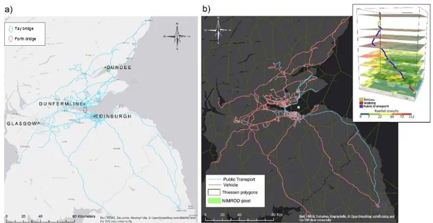
We analysed a human movement dataset where GPS devices were carried by volunteers from the

Kingdom of Fife – UK (Figure 2a) (Si

ł

a-Nowicka et al., 2016). The data were collected between the

155 

28

of September 2013 and the 10

of January 2014 as part of the GEOCROWD project (Si

ł

a-Nowicka et al., 2016), in which 6000 individuals were randomly selected by postcode address from

the voting registry (focusing on the three major towns in this region) and invited via letter to participate

in the study. In total, 206 individuals accepted the invitation and provided useable data whereby they

were tracked for two consecutive weeks within the study time spam. GPS devices recorded

160 

participant positions every five seconds, representing a very high-resolution trajectory of participant

locations. The GPS trackers were coupled with accelerometers, which turned off the GPS when the

individual was not moving Oshan

et al.

2014). The aim of the GEOCROWD project was to develop

new movement analytics methods that would allow researchers to find out as much as possible from

the actual GPS data while participants were asked to do as little as possible (i.e. the only task was to

165 

carry a GPS device and mail it back after two weeks). Therefore, very little auxiliary data were

collected and beyond gender and age of the participants, which were sourced from the electoral

register together with the address of each participant, no other demographic or ground truth data were

collected. For more details on data collection refer to Oshan

et al.

(2014).

In this paper we re-analyse the GEOCROWD data from the town (called Dunfermline; Figure 2a)

170 

175

180

185

190

195

46 were

their age

about pa

Figure

represen

Forth ro

polygons

of a NIM

corner il

cube wit

The pa

Traffic S

Stop) (S

compari

classifica

et al.

20

2.2.

We lin

linear dy

contextu

immedia

e between 35

e. As stated

articipants or

2 – a) Ea

nted by light

oad bridges r

s used to int

MROD (Met O

llustrates a t

th rainfall dat

articipant tra

Stop, Bus St

Si

ł

a-Nowicka

ng a 200 m

ation algorith

16).

Contextual

ked meteoro

ynamic trajec

ual variable

ately before

5 and 60 yea

above, apa

r their activiti

ast coast of

blue lines. T

respectively.

terpolate MID

Office's nowc

trajectory sam

ta for a

one-ajectories we

top, Train St

et al., 2016)

range from

hm (for more

data and co

ological data

ctory annota

at the time

and after the

ars old, 8 we

art from their

es were ava

f Scotland w

The green an

b) Sample

DAS (Met Of

casting syste

mple classifi

hour period.

ere classified

top, Fig. 2b)

). The classi

the recorde

e details on d

ontext integ

from ground

tion (DTA-L)

e when the

e point chro

ere between

r home addr

ailable for our

where the

nd the red e

of two move

ffice Integrat

em) product

ied into mov

d into movem

) and stop c

ification achi

ed home add

data segmen

ration

d stations an

) (Brum-Bast

GPS point

onologically.

61 and 65 y

ess, gender

r secondary

GPS data w

llipses repre

ement travel

ted Data Arc

for comparis

vement mode

ment classes

lasses (Hom

eved 85% a

dresses with

ntation and c

nd orbital sat

tos et al., 20

was collec

The DTA-L

years old, an

, and age; n

data analysis

were collect

sent the loca

modes over

chive System

son. The fram

es and displa

s (Walk, Tra

me, Work, Sh

ccuracy, wh

the home lo

lassification

ellites to mo

016), a metho

cted by inte

method acco

nd 27 did no

no further inf

s.

ted, and tra

ations of the

rlaid by the T

m) data and o

me in the rig

ayed in a sp

ain, Bus and

hopping, Un

ich was asse

ocation foun

refer to

Sila-ovement data

od that estim

erpolating the

ounts for the

ot declare

formation

ajectories

Tay and

Thiessen

one pixel

ght upper

pace-time

Vehicle

identified

essed by

nd by the

-Nowicka

a through

mates the

rate-of-Manuscript accepted to 

Computers, Environment and Urban Systems

, May 2018 

change between contextual layers, producing more realistic values for interpolated meteorological

data, and it also deals with the difference between temporal resolutions of the datasets (Brum-Bastos

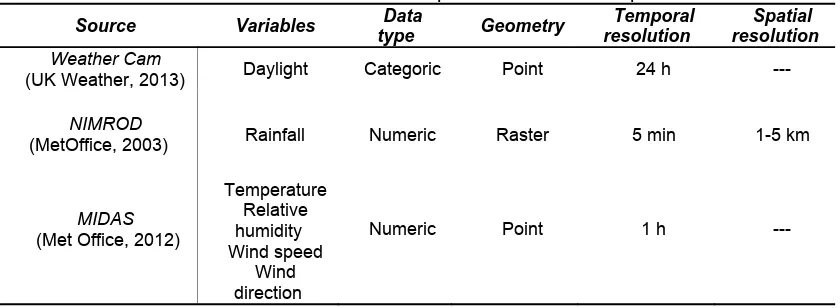
et al. 2017). We collated multiple sources of contextual data on weather (Table 1).

200 

Table 1– Contextual datasets with respective sources and specifications.

Source Variables Data

type Geometry

Temporal resolution

Spatial resolution Weather Cam

(UK Weather, 2013) Daylight Categoric Point 24 h ---

NIMROD

(MetOffice, 2003) Rainfall Numeric Raster 5 min 1-5 km

MIDAS (Met Office, 2012)

Temperature Relative humidity Wind speed

Wind direction

Numeric Point 1 h ---

We associated MIDAS data with trajectory points using Thiessen Polygons around each

meteorological station (n = 109, Fig 2b). From the MIDAS meteorological variables we also derived

the apparent temperature (

, which considers the combined effects of temperature, humidity and

205 

wind (Steadman, 1994).

0.33 ∗

0.70 ∗

4.00

(1)

Here

is the air temperature in °C; is the water vapour pressure in hPa calculated from the

relative humidity and temperature; and

is the wind speed in m/s.

The Weather Cam data was used to calculate dusk, sunset, sunrise and dawn times (for a central

210 

location in the study area) as at this latitude daylight length varies by approximately 4.5 hours from

September to January. Daylight categories were annotated to trajectories according to the following

rules: Morning Twilight (MT) for fixes recorded in the period between dawn and sunrise, Day Light (DL)

for fixes recorded between sunrise and sunset, Evening Twilight (ET) for fixes recorded between

sunset and dusk, Night (NI) for fixes recorded between dusk and dawn.

215 

2.3. Trajectory

sequencing

Tsay, 2000). However, most phenomena are multidimensional and require multiple alphabets. This

means that each dimension gets its own bespoke alphabet and instead of having the data object

represented as one sequence, the object now has as many different sequences as there are

dimensions, which are called channels (therefore the name Multi-Channel Sequence Analysis). The

alignment, i.e. similarity, then needs to be calculated across all channels along the time axis (Gauthier

225 

et al., 2010). This multi-channel approach is therefore a shift from looking at individual units towards

analysing context, connections and events (Abbott, 1995).

We created several bespoke alphabets, one for movement mode (e.g., walking and driving) and one

for each weather variable in our data. For this, we had to translate the GPS track of each participant

into a multi-channel sequence consisting of time units, to which the characters were assigned (figure

230 

3). Weather conditions were categorized to create weather-based alphabets (Table 2). Rainfall was

classified based on the UK Met Office scale for rainfall intensity, Wind Speed according to an

adaptation of the Beaufort scale (Royal Meteorological Society, 2017), wind direction according to the

cardinal and collateral points, apparent temperature according to the VDI (2008) thermal perception

scale, humidity and temperature according to the 1991-2000 seasonal climate normals for

235 

Dunfermline from Jenkins

et al.

(2009). Climate normals are a three-decade average of weather

variable commonly used to characterize local climates (Ayoade, 1986).

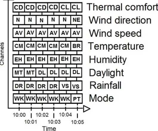
The multi-channel sequences were then generated for each volunteer and day (illustrated in Figure

3) by taking the modal weather condition (for each variable described in Table 2) and movement

mode for each 1-minute interval for each participant. To each time unit we assigned descriptors for

240 

the weather variables and the respective movement mode, which are linked to the descriptor for the

following time unit building multiple chronologically arranged strips. These sequences can be

analysed alongside strips of contextual variables to understand not only the responses to specific

variables, but also to different combinations of those variables and the identification of patterns

relative for specific age groups, gender or other profiling information. The number of channels in a

245 

250

255

260

Figure

to one o

We calc

minute (

group of

of places

indicates

while an

average

and on

amount

participa

this, we

Manuscrip

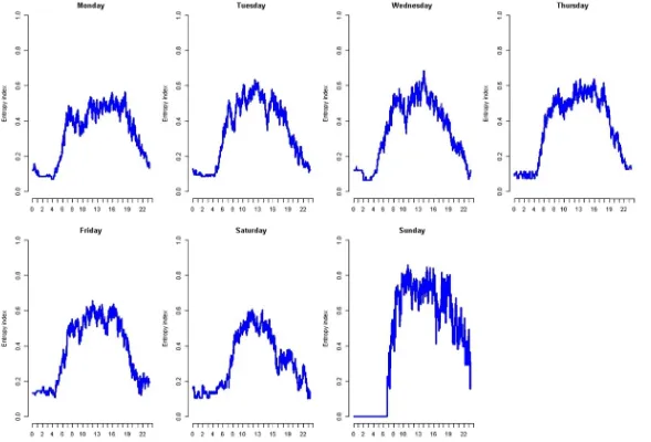
3 - A multi-c

of the meteor

culated the e

(Billari, 2001

f sequences

s and travel

s an even d

n EI closer to

e time expend

each day of

of time spen

ant, keeping

calculated th

pt accepted t

channel sequ

rological varia

entropy index

). The EI is a

(Gabadinho

modes acro

distribution o

o zero indica

diture at hom

f the week. T

nt in each m

in mind that

he mean for

to 

Computer

uence for a p

ables and m

x (EI) for the

a measure o

o et al., 2009

ss the week

of a contextu

ates a high le

me, socialisin

The average

movement m

each state

the gender o

rs, Environme

participant ov

ovement mo

e movement

of the comple

9),which in ou

and hours o

ual variable

evel of assoc

ng, shopping

e time expen

mode and div

in our seque

of participant

ent and Urba

ver a five-min

odes for that

t mode chan

exity induced

ur case can

of the day. In

across mov

ciation with o

, walk, public

nditure was c

viding it by th

ences corres

ts (male, fem

an Systems

, M

nute period,

minute of the

nnel for all se

d by the distr

be used to

our analysis

vement mode

one mode. W

c transport a

calculated b

he total GPS

ponded to o

male).

May 2018 

each channe

e day.

equences of

ribution of st

observe the

s, an EI clos

es (alphabet

We also look

and vehicle b

by first comp

S active time

one minute. F

el relates

Table 2 – Alphabets for meteorological variables used as contextual data with respective ranges and description. Letters in each alphabet are defined based

265

on standard meteorological classifications (see text for more details).

Thermal perception (°C) Rainfall (mm/h) Wind coming from direction (°)

Letter Description Range Letter Description Range Letter Description Range

VC Very Cold <= -39 DR Dry 0 N North > 337.5 - 22.5

CD Cold >-39 - -26 VS Very Slight >0 - 0.5 NE North East >22.5 -67.5

CL Cool >-26 - -13 SL Slight >0.5 – 1 E East > 67.5 -112.5

SC Slightly Cool >-13 - 0 LM Low Moderate >1 – 2 SE South East >112.5 - 157.5

CF Comfortable >0 - 20 MO Moderate >2 – 4 S South >157.5 – 202.5

SW Slightly Warm >20 - 26 HV Heavy >4– 10 SW South West >202.5 – 247.5

W Warm >26 – 32 VH Very Heavy >10 - 50 W West _292.5 > 247.5 –

H Hot >32 – 38 VI Violent > 50 NW North West >292.5 – 337.5

VH Very Hot >38

Humidity (%) Temperature (°C) Wind Speed (m/s)

Letter Description Range Letter Description Range Letter Description Range

EH Extremely High >90 EL Extremely Low <=5 CM Calm <= 3

AA Above Average >85 -90 AN Average minimum > 5-7 BR Breeze >3 - 14

AV Average >80 -85 AV Average Average >7 -10 GA Gale >14 - 24

BA Below Average >75 -80 AX Average Maximum >10 - 13 ST Storm >24

LW Low >70 -75 EH Extremely High >13

Manuscript accepted to 

Computers, Environment and Urban Systems

, May 2018 

2.4.

Context-Aware Similarity Analysis (CASA)

2.4.1. Multi-channel Sequence Analysis (MCSA)

270 

We divided our analysis into two streams, by separately analysing travel modes (walk, public

transport and vehicle) and places (home, social places and shopping), since the choice of travel mode

and of staying in a place are not necessarily affected in the same way by weather (Derrick Sewell,

Kates, & Philips, 1968). When the destination is obligatory, such as work, people are more likely to

change their travel mode, for example, driving to work instead of walking under heavy rain; however,

275 

if the destination is linked to leisure, such as shopping, people might simply postpone the task instead

of changing the travel mode to get there (Connolly, 2008; Zivin, 2014). We further split the analysis

into weekdays and weekends to reflect different movement motivations (for example, travel to work

during workdays is usually obligatory regardless of weather conditions while people have more

voluntary choices about their mobility during weekends).

280 

Sequence analysis requires cost matrices, which were computed separately for travel modes and

places and for weekends and weekdays. We used the optimal matching (OM) distance to compute

similarity between sequences as this method has shown potential for identifying groups with matching

movement behaviour (De Groeve et al., 2016). The distance between two sequences is assessed by

quantifying their differences based on a matrix with the costs for substituting, deleting or inserting

285 

letters to transform one sequence into the other. The substitution costs are given by symmetrical

matrices that represent the costs of transitioning between each pair of states in the alphabet

(Gabadinho et al., 2009). In our case, the costs for transitions between the states of travel modes,

places, wind speed and wind direction were computed using transition rates calculated from the

sequences for computing the cost matrices, as shown in Equation 2.

290 

,

1

,

,

(2)

Here

,

is the substitution cost,

,

is the transition rate from state to .

The costs for transitions between the states of thermal comfort, temperature, humidity, daylight and

rainfall were defined by ordering the classes of each variable (alphabets) by their intensity and

calculating the cost to replace one class by another with Equation 3.

295 

Here

,

is the cost between the classes and with intensity order

and

1

, and is the

number of classes for that variable (size of the alphabet). The cost for replacing null values by any

other class (insertion) was zero and likewise to substitute any other class by null (deletion), because

for our study they are related to periods for which we had no information on the participant’s

300 

movement. This procedure resulted in ten cost matrices, one for each weather variable, two for travel

modes and two for places (weekdays and weekend).

The cost matrices are then used to calculate the optimal match (OM) score, for example, given an

alphabet with size , pick sequences and based on alphabet . The sequences are aligned in

time and the OM cost is calculated by summing up the costs of substitutions

, deletions and

305 

insertions

d

needed to modify the sub sequences of , so that it turns into . The OM is the less

costly and is computed using Equation 4, in which each line defines a possible OM score for two sub

sequences, depending on which of the procedures, insertion, deletion or substitution, is cheaper

(Gauthier et al., 2010).

,

1,

1

1,

d

,

1

d

(4)

310 

Here

1,

1

represents the OM score of a subsequence containing the

1

to

1

characters

of sequence against a subsequence containing

1

to

1

in sequence (Gabadinho et al., 2009;

Gauthier et al., 2010). The OM cost is computed for each channel between all multi-channel

sequences and the cost between two multi-channel sequences is the summed costs between their

channels. We calculated the OM distances simultaneously considering three channels for wind:

315 

movement mode, wind speed and wind direction; and two channels for the remaining weather

conditions, where the places or the travel modes were always the first channel and the variables were

considered in turns as the second channel. A by dissimilarity matrix, where is the number of

sequences, represents the level of alignment between each two multi-channel sequences, i.e., a

similarity measure between two moving people.

320 

2.4.2. Cluster analysis & typology

Manuscript accepted to 

Computers, Environment and Urban Systems

, May 2018 

dissimilarity matrix for each weather variable for both travel modes and places. We used Ward’s

clustering, a hierarchical bottom-up algorithm that computes dissimilarities between two groups as the

325 

increase in the error sum of squares after merging those groups. The algorithm starts with each

sequence as their own group and successively merges them into clusters based on the minimum

increase in the error sum of squares, until it becomes a single cluster (Murtagh & Legendre, 2011).

For selecting the optimal number of clusters, we used the Calinski-Harabaz Index (CHI) (Calinski &

Harabasz, 1974) that considers the within and between groups dispersion as shown in Equation 5.

330 

(5)

Here and are the within and between group dispersion matrices, the trace of is the sum of

the within cluster variance and the trace of is the sum of the between cluster variances; a higher

CHI indicates a better data partition (Ahmed, 2012), because it shows that the within group distances

are lower and the between groups distances are higher. We varied the number of clusters from the

335 

number of sequences (i.e. the maximum possible number of clusters, if every sequence is allocated to

its own cluster) to one and used the configuration with highest CHI, except where the maximum CHI

resulted in individuals’ clusters, to assign the multi-channel sequences into their final clusters. The

combination of values of weather and movement modes in each cluster then defined a type of the

group. Note that the types are not consistent between variables, i.e., we found different clusters for

340 

each weather variable, thus the typology is specific for each variable.

We then looked at the distribution of the proportion of time spent in different travel modes and

places for the weather conditions associated with each cluster. We expected this would give insights

into the different behavioural patterns in individuals related to weather (i.e., an overall picture of the

effects of the weather conditions within each cluster on movement modes). We tested the significance

345 

of the differences using Kruskal-Wallis and Levene’s tests and we assumed that a statistically

significant difference between medians or variances of each cluster was enough evidence to support

the existence of different behavioural groups.

We further used discrepancy analysis to verify if and how behavioural groups were related to age

and gender. This method evaluates the strength of the association between the groups of sequences

350 

(6)

Here

is the share of discrepancy,

is the sum of square distances within the age or gender

groups, and

is the total sum of square distances between all sequences (Batagelj, 1988).

355 

3. Results

3.1. Trajectory

sequencing

The different movement modes for each participant for each day of the week are shown in Figure 4,

most sequences start between six and eight in the morning and have a minimum of 58% and a

maximum of 98% of missing data, i.e., minutes for which the GPS tracker was off and movement

360 

modes are unknown (white gaps in Figure 4). The entropy index (EI) (Figure 5) provides some insight

into participants daily movement behaviour. The EI increases between 4:00 am and 7:00 am on

weekdays, but only rises between 8:00 am and 10:00 am on weekends, indicating higher diversity of

movement modes earlier on weekdays. Sunday has the highest EI and similarly to Saturday, it drops

and rise between 3:00 pm and 6:00 pm.

365 

The average time spent (AVTS) walking did not change substantially across weekdays and

between genders (Figure 6). The AVTS at home varied throughout the week, being the highest on

Sunday and lowest on Wednesday for both genders (dashed orange lines on Figure 6). The low

values on Wednesday might be related to the higher average time spend socializing in comparison to

other days of the week (dashed red lines on Figure 6). Moreover, women seem to spend more time

370 

375

re

d

Manusc

Figure 4 - Sequ

eported in white.

does not always in

ript

accepted

to

C

ences of moveme

For each day, the

ndicate the same

Computers,

Enviro

ent modes for eac

e sequences are

individual).

onment

and

Urban

ch day of the wee

ordered by length

n

Systems

,

May

2

ek by participant (v

h, but orderings a

018

vertical axis) and

m

380

Figure 5 - Entro

movement mode

opy index (EI) by

at that time (lowe

day of the week

er diversity), whil

and by hour of th

le an EI close to

he day (horizontal

one indicates si

l axis), an EI clos

milar proportion o

se to zero indicate

of people on the

es that most peop

different movem

ple are in the sam

ment modes (high

fe

Manusc

Figure 6 - Aver

emales (22 ≤ n ≤

ript

accepted

to

C

rage time expend

33) and the secon

Computers,

Enviro

diture and trend o

nd row to males (5

onment

and

Urban

over the week (da

54 ≤ n ≤ 70).

n

Systems

,

May

2

ashed lines) by m

018

385

390

395

400

405

3.2.

3.2.1.

Overal

(Figure

homoge

to the w

shown b

within g

results in

On we

variables

(Figure

travel m

humidity

highest

discernib

Figure

performe

weekend

sequenc

Context-Aw

Cluster ana

ll the CHI w

7) indicating

enous movem

weekend. Thi

by the highe

roup distanc

n a higher op

eekdays the

s but relativ

7 left). This

modes and re

y as a proxy

discernibility

bility was ass

7 -

Calinski-ed on weath

d. The repor

ces.

ware Similar

alysis & typo

was higher o

g the existe

ment behavio

s could also

er EI; more

ces making

ptimum numb

e CHI follow

ve humidity,

indicates a

elative humi

for rainfall to

y for travel

sociated with

-Harabaz ind

her variables

rted CHI is

ity Analysis

ology

on weekdays

ence of a c

our within th

be reflective

variety migh

more difficul

ber of cluste

wed a simila

for which th

stronger dis

idity on wee

o plan their j

mode diffe

h temperatur

dex (solid line

s for travel

divide by te

s (CASA)

s for all wea

clear division

hese groups

e of the high

ht lead to low

lt to identify

r, as seen on

ar pattern fo

he index wa

stinction bet

ekdays, whic

journeys. Re

rences durin

re, rain and c

e) and optim

modes (gre

n and refers

ather variabl

n amongst b

regarding th

her diversity

wer separab

group’s res

n the weeken

or travel mo

as about two

tween the tw

ch might be

elative humid

ng the wee

comfort durin

mal number o

een) and pla

s to the num

es for trave

behavioural

he weather e

of activities d

bility between

sponses to w

nd chart (Fig

des and pla

o times high

wo behaviou

related to p

dity, rain and

k, while for

ng the weeke

f clusters (da

aces (red) o

mber of clust

el modes an

groups and

effects in com

during the w

n groups an

weather. This

gure 7 right).

aces for all

her for trave

ural groups r

people using

d comfort sho

r places the

end.

ashed line) fo

on weekdays

ters used to

d places

a more

mparison

weekends

nd higher

s usually

weather

el modes

regarding

g relative

owed the

e highest

or MCSA

s and on

Manuscript accepted to 

Computers, Environment and Urban Systems

, May 2018 

Next, we present some of the more interesting findings while the remaining set of results can be

found in the appendix. The typologies are specific for each variable, i.e., Type 1 for wind is not the

same as type 1 for rainfall. The analysis of shared discrepancy did not show significant correlation

between the behavioural clusters and gender or age groups, all SD were lower than 0.01 with

non-410 

significant p-values (

α

= 0.1). Significant values for Levene’s (L) and Kruskal-Wallis’ tests (K) are

reported on the heading of each graph on the pictures by the following symbology: *** for

α

= 0.001, **

for

α

= 0.01, * for

α

= 0.5, . for

α

= 0.1.

3.2.2. Wind

Figure 8 shows the clusters for MCSA on wind on weekdays (Figure 8A) and weekends (Figure 8B).

415 

The top boxplot shows the distribution of the GPS active time spent under wind blowing from each

direction and the middle one shows the distribution of the GPS active time spent under different wind

intensities. Both boxplot panels are divided into Type 1 and Type 2, which refer to the two clusters

found by the MCSA analysis and for which the distribution of the GPS active time in different travel

modes is shown on the boxplot panel at the bottom. This boxplot shows the difference between

420 

groups with different distribution of time spent on travel modes, while the remaining panels describe

the wind conditions encountered within those groups. There were no significant differences on the

average time spent on different travel modes on weekdays under different wind conditions (Figure 8A),

on the weekend however we found significant differences on the average time expenditure in public

transport and vehicle (Figure 8B). CASA clustering showed a significantly lower use of public

425 

transportation with concurrent increase on the use of vehicles under more windy conditions coming

from North-East, North-West and South-West (Type 2).

430 

440

445

450

455

Figure

weekend

respectiv

two pan

each tra

show the

from Kru

Figure

The top

direction

intensitie

which re

active tim

differenc

panels

significa

socialisi

Type 1,

A

8 – Clusters

ds (B). The

ve proportio

els at the bo

avel mode b

e average an

uskal-Wallis’

9 shows the

boxplot sho

n and the mid

es. Both box

efer to the c

me in differe

ce between

describe the

ant difference

ng on the we

Type 3 and

A)

s for MCSA o

four top pan

ns of GPS a

ottom show b

by the wind t

nd the contin

test.

e clusters for

ows the distr

ddle one sho

xplot panels

clusters foun

ent activities

groups with

e wind con

es in the ave

eekend (Figu

Type 4 are v

on wind spee

nels describe

active time s

boxplots with

types descri

nuous line the

r MCSA on w

ribution of th

ows the distr

are divided i

nd by the MC

is shown on

different dis

ditions enco

rage time ex

ure 9). There

very similar i

ed, wind dire

e the wind co

pent under t

h the distribu

bed on the

e median. L

wind on week

he GPS activ

ribution of th

into five type

CSA analysi

n the boxplot

stribution of

ountered wit

xpenditure at

e were five c

n terms of tim

ection and tra

onditions wit

the classes o

tion of propo

panels abov

reports sign

kdays (Figure

ve time spen

e GPS activ

es on weekd

is and for w

t panel at the

time spent o

thin those g

t home and s

clusters base

me spent at

B) 

avel modes o

hin each clu

of wind spee

ortional GPS

ve. The dash

ificance from

e 9A) and we

nt under win

e time spent

ays and two

which the dis

e bottom. Th

on activities,

groups. For

shopping du

ed on wind d

places and t

on weekdays

uster (Types)

ed and direc

S active time

hed line on

m Levene’s te

eekends (Fig

d blowing fr

t under differ

o types on we

stribution of

his boxplot sh

, while the re

places, the

ring the wee

during weekd

they do not s

s (A) and

) and the

tion. The

spent on

boxplots

est and K

gure 9B).

rom each

rent wind

eekends,

the GPS

hows the

emaining

ere were

ek, and in

460

465

470

475

480

because

time spe

CASA c

under m

not show

the time

Figure

weekend

respectiv

two pan

places b

average

Kruskal- 

3.2.3.

Figure

10B). Th

intensitie

which re

 A

Manuscrip

e of its smal

ent at home

lustering on

more windy co

w any prevai

.

9 – Cluste

ds (B). The

ve proportio

els at the bo

by the wind

e and the co

-Wallis’ test.

Rain

10 shows th

he top boxp

es. The boxp

efer to the c

A)       

pt accepted t

l number of

with concur

weekend sh

onditions com

ling direction

rs for MCSA

e four top p

ns of GPS a

ottom show b

types descr

ontinuous line

he clusters fo

plot shows th

plot panel is

clusters foun

to 

Computer

participants

rrent increas

owed a sign

ming from NE

n and its stre

A on wind s

panels desc

active time s

boxplots with

ribed on the

e the media

or MCSA on

he distributio

divided into

nd by the MC

rs, Environme

(n = 7); Typ

se of time sp

ificant decre

E, NW and S

ngth alternat

speed, wind

cribe wind c

pent under t

h the distribu

e panels abo

n. L reports

rainfall on w

on of the GP

o three types

CSA analysi

ent and Urba

pe 2 howeve

pent shoppin

ase on the p

SW (Type 2).

tes between

direction an

conditions w

the classes o

tion of propo

ove. The da

significance

weekdays (Fi

PS active tim

s on weekda

is and for w

 B) 

an Systems

, M

er, showed a

ng under mo

proportional t

Whereas w

calm and ga

nd places on

within each

of wind spee

ortional GPS

ashed line on

e from Leven

gure 10A) an

me spent un

ays and four

which the dis

May 2018 

a lower prop

ore windy co

time spent so

weekend Typ

ale for aroun

n weekdays

cluster (Typ

ed and direc

S active time

n boxplots s

ne’s test and

nd weekend

nder differen

types on we

stribution of

portion of

onditions.

ocialising

pe 1 does

d 88% of

(A) and

pes) and

tion. The

spent on

show the

d K from

s (Figure

nt rainfall

485

490

495

500

active tim

the diffe

remainin

significa

different

average

more dr

rainfall (

decreas

Figure

two top

of GPS

the distr

on the p

median.

Figure

11B). Th

intensitie

     A

me in differe

erence betwe

ng panels de

ant difference

t rain conditi

e time spent

rier condition

(Type 3) with

e on walking

10 – Cluste

panels desc

active time s

ribution of pr

panel above

L reports sig

11 shows th

he top boxp

es. The box

A)      

ent travel mo

een groups

escribe the

es in the ave

ions (Figure

in public tra

ns (Type 1 a

h a concurren

g.

ers for MCSA

ribe the rain

spent under

roportional G

e. The dashe

gnificance fro

he clusters fo

plot shows th

plot panel is

odes is show

with differen

rainfall cond

erage time ex

10), on we

ansport (Figu

and Type 2)

nt, but not st

A on rain and

conditions w

the rainfall c

GPS active tim

ed line on b

om Levene’s

or MCSA on

he distributio

s divided into

wn on the box

nt distributio

ditions encou

xpenditure fo

eekdays how

ure 10). CA

), public tran

tatistically sig

d travel mod

within each c

classes. The

me spent on

boxplots sho

s test and K f

rainfall on w

on of the GP

o three type

xplot panel a

on of time sp

untered with

or different t

wever we fou

ASA clusterin

nsport is sign

gnificant, inc

des on week

cluster (Type

two panels

each travel

ow the avera

from Kruskal

weekdays (Fi

PS active tim

s on weekda

 B) 

at the bottom

pent on trav

in those gro

ravel modes

und significa

ng showed th

nificantly les

crease on the

days (A) and

s) and the re

at the bottom

mode by the

age and the

-Wallis’ test.

gure 11A) an

me spent un

ays and six

m. This boxpl

vel modes, w

oups. There

s on weeken

ant difference

hat in comp

ss used und

e use of veh

d weekends

espective pro

m show boxp

e rain type d

e continuous

.

nd weekend

nder differen

types on we

ot shows

while the

were no

ds under

es in the

arison to

er heavy

icles and

(B). The

oportions

plots with

described

s line the

s (Figure

nt rainfall

505

510

515

520

525

active tim

differenc

panels

differenc

under di

condition

other ra

more tim

under pr

rain con

Figure

panels d

active ti

distribut

above. T

significa

On we

outliers.

time is s

     A

Manuscrip

me in differe

ce between

describe th

ce for place

ifferent rain c

ns (Type 1),

in states (Ty

me at home u

redominantly

ditions (Type

11 – Cluste

describe the

me spent un

ion of propo

The dashed

ance from Lev

eekends, Typ

Under heav

spent at hom

A)       

pt accepted t

ent activities

groups with

e rainfall c

s was on th

conditions (F

a second cl

ype 2) and a

under violent

y dry conditio

e 2).

ers for MCSA

rain conditio

nder the rain

ortional GPS

line on boxp

vene’s test a

pe 5 and Typ

vy rainfall (Ty

me under pre

to 

Computer

is shown on

different dis

conditions en

he average t

Figure 11). O

uster with dr

a third cluste

t rain (Type

ons (Type 1

A on rain and

ons within ea

nfall classes

active time

plots show th

and K from K

e 6 have suc

ype 3) there

dominantly d

rs, Environme

n the boxplot

stribution of

ncountered

time expend

On weekdays

ry conditions

er with violen

3), but surpr

) in compari

d places on w

ach cluster (T

s. The two p

spent on pla

he average a

Kruskal-Wallis

ch a sparse

is a higher a

dry condition

      B

ent and Urba

t panel at the

time spent o

within thos

diture at hom

s we found o

s but an even

nt rain (Type

risingly peop

ison when th

weekdays (A

Types) and th

panels at the

aces by the

and the conti

s’ test.

number of m

average time

ns, even with

B) 

an Systems

, M

e bottom. Th

on activities,

e groups. T

me on week

ne cluster w

n distribution

3). As exp

le also spen

here is a mix

A) and weeke

he respective

e bottom sho

rain type de

inuous line t

members that

e expenditure

the remaini

May 2018 

his boxplot sh

, while the re

The only s

kends and w

with predomin

n of time amo

pected, peop

d more time

x of dry and

ends (B). The

e proportions

ow boxplots

escribed on t

the median.

t we conside

e at home, w

ng time bein

hows the

emaining

ignificant

weekdays

nantly dry

ongst the

ple spend

at home

different

530

535

540

545

evenly d

1) showe

3.2.4.

Figure

(Figure

condition

which re

active tim

the diffe

remainin

significa

weekday

Figure

The two

proportio

show bo

daylight

the med

   A

distributed am

ed the highe

Daylight

12 shows

12B). The to

ns. The box

efer to the c

me in differe

erence betwe

ng panels de

ant difference

ys under diff

12 – Cluste

o top pane

ons of GPS

oxplots with t

type describ

ian. L report

A)      

mongst the o

er time expen

the clusters

op boxplot sh

plot panel is

clusters foun

ent travel mo

een groups

escribe the d

es on the ave

ferent dayligh

ers for MCSA

els describe

active time

the distributio

bed above. T

ts significanc

other rain co

nditure at hom

s for MCSA

hows the dist

s divided into

nd by the MC

odes is show

with differen

daylight cond

erage time ex

ht conditions

A on dayligh

daylight co

spent unde

on of propor

The dashed li

ce from Leve

onditions (Typ

me.

on daylight

tribution of th

o three types

CSA analysi

wn on the box

nt distributio

ditions enco

xpenditure fo

(Figure 12).

ht and travel

onditions w

er the classe

rtional GPS a

ine on boxpl

ne’s test and

pe 2 and Typ

on weekda

he GPS activ

s on weekda

is and for w

xplot panel a

on of time sp

untered with

or different tr

.

modes on w

ithin each

es of dayligh

active time s

ots show the

d K from Kru

  B) 

pe 4); the dr

ays (Figure

ve time spen

ays and two

which the dis

at the bottom

pent on trav

hin those gro

ravel modes

weekdays (A

cluster (Typ

t. The two p

spent on eac

e average an

skal-Wallis’ t

riest conditio

12A) and w

nt under diffe

types on we

stribution of

m. This boxpl

vel modes, w

oups. There

on weekend

A) and weeke

pes) and re

panels at the

ch travel mod

nd the contin

test.

ns (Type

weekends

erent light

eekends,

the GPS

ot shows

while the

were no

ds nor on

Manuscript accepted to 

Computers, Environment and Urban Systems

, May 2018 

Despite not being statistically significant, less daylight time resulted in less time walking (Type 3)

550 

compared to more time walking under more daylight hours (Type 1 and Type 2). A similar decrease is

observed on the time expenditure in public transport, with a concurrent increase on time expenditure

in vehicles. This trend reverses on weekends, in which walking and public transport are more

prominent than the use of vehicle in a group exposed to more night hours (Type 2), while the use of

vehicles prevails in a group with more daylight hours (Type 1).

555 

Figure 13 shows the clusters for MCSA daylight on weekdays (Figure 13A) and weekends (Figure

13B). The top boxplot shows the distribution of the GPS active time spent under different light

conditions. The boxplot panel is divided into three types on weekdays and two types on weekends,

which refer to the clusters found by the MCSA analysis and for which the distribution of the GPS

active time in different activities is shown on the boxplot panel at the bottom. This boxplot shows the

560 

difference between groups with different distribution of time spent on activities, while the remaining

panels describe the daylight conditions encountered within those groups. The analysis for daylight

and places, was significant for all places both on weekend and weekdays. There are 3 daylight types

on weekdays, Type 1 has more daylight, Type 2 is the one with more night time and Type 3 is an

almost even mix of day and night (Figure 13). Type 1 has less time spent at home than Type 2,

565 

however we are unsure why the time expenditure at home is the lowest for Type 3. There is less

shopping and socialising in the group with more night hours (Type 2). On weekends (Figure 13 B).

more time is spent at home under brighter conditions (Type 2), while under lower light conditions

(Type 1) more time is spent shopping and socialising.

570 

580

585

590

595

Figure

top pane

active ti

distribut

The das

significa

4.

The rece

opportun

behavio

particula

identifyin

other ty

direction

active ti

   A)     

13 – Cluste

els describe

ime spent u

ion of propo

shed line on

ance from Lev

Conclusion

ent widespre

nities for de

ur and envi

ar the choice

ng groups of

pes of move

n), rainfall, d

me spent o

rs for MCSA

daylight con

under dayligh

ortional GPS

n boxplots s

vene’s test a

ns and discu

ead availabil

eveloping n

ironment. W

e of travel m

f specific be

ement and

daylight, com

n travel mo

A on daylight

ditions within

ht classes.

active time

show the av

and K from K

ussion

ity and quali

ew method

We were inte

mode and tim

haviour unde

contextual d

mfort, relative

des (walk, p

and places

n each cluste

The two pa

spent on pl

verage and

Kruskal-Wallis

ity of geospa

s to unders

erested on

me spent on

er certain we

data. We inv

e humidity a

public transp

       B)

on weekday

er (Types) an

anels at the

aces by the

the continu

s’ test.

atial data on

stand the i

how weathe

activities. O

eather condi

vestigated th

and tempera

port, vehicles

s (A) and we

nd respective

bottom sho

daylight typ

uous line the

movement a

nteractions

er affects hu

Our methodo

tions, and it

he impact of

ature, on the

s) and place

eekends (B).

e proportions

ow boxplots

pe describe

e median. L

and context

between m

uman move

ology was ef

can be exp

f wind (stren

e proportion

es (home, s