A Combined Probabilistic and Optimization Approach for Improved Chemical Mixing Systems Design

doi:10.4236/eng.2011.36077 Published Online June 2011 (http://www.SciRP.org/journal/eng)

A Combined Probabilistic and Optimization Approach for

Improved Chemical Mixing Systems Design

Matthew J. Opgenorth1, William E. McDermott2, Peter Laz1, Corinne S. Lengsfeld1* 1

Department of Mechanical and Materials Engineering, University of Denver, Denver, USA

2

Applied Research and Technology Institute, University of Denver, Denver, USA E-mail: [email protected]

Received March 17, 2011; revised April 12, 2011; accepted April 17, 2011

Abstract

A design analysis of a mixing nozzle was performed using a combination of probabilistic and optimization techniques. A novel approach was utilized where probabilistic analysis was used to reduce the number of geometric constraints based on sensitivity factors. An optimization algorithm used only the most significant parameters to maximize mixing. A second probabilistic analysis was performed after optimization was com-plete in order to quantitatively predict the effects of manufacturing tolerances on mixing performance. This process for automated design is attractive over full parameter optimization techniques due to the computa-tional efficiency resulting from an intelligent reduction in evaluated variables.

Keywords:Probabilistic Design, Optimization Design, Tolerance Design, Computer-Aided Design

1. Introduction

Computational fluid dynamics (CFD) analyses, with software packages like Fluent™ (ANSYS, Inc.), have become accepted techniques for solving complex fluid flows using numerical implementation of fluid mechan-ics principles. CFD-driven optimization has been ex-plored by several researchers [1-3]. Peigin et al. has proposed a design tool that implements multi-constrained optimization of shape design driven by Genetic Algo-rithms (GA) coupled with CFD. The benefit to GA is that they can handle a large number (20+) of design variables; however, with a large number of constraints, GA are computationally expensive. Peigin et al. reports 15-18 hours for a single point optimization and on average 8-12 optimization steps [1]. A similar multi-constrained opti-mization strategy has been implemented on a ship’s hull. Again the downside is the time constraints, where they report approximately 10 days for 20 shape generations on a PC-based cluster [2]. Many researchers are using these GA’s in order to optimize a system with numerous variables.

GA’s have also been used by Carroll (1996) for the modeling of complex chemical mixing systems. The GA was coupled with the Blaze II code [4]. The Blaze II code can address up to 500 chemical reactions and 40 species. It also contains 1-D fluid dynamic equations, with mixing

terms derived from 2-D equations, that can be used to model axis symmetric and 2-D flow fields [4]. The GA used 5 parameters with either 32 or 16 discrete possibili-ties resulting in approximately 2 million permutations. Even with a 2-D model and only 5 variable parameters the GA required 8 days of continuous runtime [3].

num-ber of constraints through probabilistic analysis, as well as, assessing the impact of manufacturing tolerances.

2. Methodology

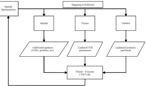
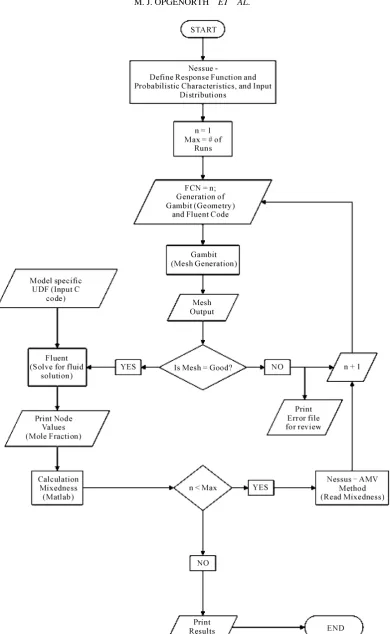
Currently, there is no commercially available tool in in-dustry to perform fluid mechanics analyses, optimization and probabilistic analysis in the proposed integrated manner. There are however, software packages that can execute individual components of the process. Our ap-proach is to use commercially available CFD, probabilis-tic and optimization software and interface them together with custom scripting. The probabilistic software, or op-timization routine, manages the CFD code by importing any number of variables within ranges and/or distribu-tions set by the user. Figure 1 and 2 show a diagram linking the processes mentioned above.

2.1. CFD Model

The CFD software used for the simulations was Fluent™ Version 6.3.26 [5]. It is a widely used computational software package for modeling fluid flow and heat transfer in complex geometries. Easy mesh generation and ability to refine or coarsen the mesh autonomously based on the flow solution are just some of the features that make this CFD package extremely versatile and

ideal for automation. Gambit® was the pre-processor used for the solid modeling and mesh generation.

The algorithm employed was the pressure-based Navier-Stokes solution algorithm. Typically, this algo-rithm is used for low velocity incompressible flows, which fits this case where the flow velocity is about 83 m/s. The momentum equation provides the velocity field and the density is calculated from the equation of state. Other governing equations include energy and species conservation. The turbulence model chosen was the standard k-epsilon turbulence model. This model is ro-bust and suitable for initial iterations, initial alternative design screenings, and parametric studies. The k-epsilon model will be ideal for the automated analysis where many different shapes will be analyzed. A no-slip boun-dary condition was placed at the walls. The primary inlet utilized a user-defined function (UDF) that modeled a fully developed fluid flow.

Definition of the boundary conditions is critical to both accuracy of the model and computational efficiency, the importance of which should not be under estimated when venturing into optimization and probabilistic anal-ysis. Considerable attention was paid to identifying the best algorithmic parameters in order to achieve conver-gence in the minimum number of iterations, reliably, and with physically correct solutions regardless of geometry. It is also noteworthy to mention that this process was

carried out in parallel on 8 processors in order to reduce computational time.

2.2. Probabilistic Model

As uncertainty is inherent in physical systems, a proba-bilistic analysis model input variables as distributions and then predicts a distribution of performance. Based on the distribution of performance, sensitivity and impor-tance factors are used to identify critical parameters. The probabilistic software, Nessus®, implements a variety of probabilistic methods that vary in efficiency and accura-cy of the solution. The most commonly used probabilis-tic method is Monte Carlo [6]. The Monte Carlo method generates random values for each variable according to its distribution and then predicts the distribution of per-formance through repeated trials. As the accuracy of the prediction is dependent on the number of trials per-formed, the Monte Carlo method is computationally ex-pensive. The mean-value (MV) family of methods are approximate, but considerably more efficient than the Monte Carlo method. They create a mean-based response function and compute the most probable point (MPP), which is the shortest distance from the origin to the limit state surface and represents the combination of stochastic variables resulting in a specific level of performance [6]. In this study, the Advanced Mean Value (AMV) method was applied, which uses a higher order approximation to determine the MPP [7]. The number of trials used for the AMV method is 1 + the number of variables + the num-ber of probability levels desired [7]. While the AMV method is a discrete and approximate solution, it has shown excellent agreement with Monte Carlo analysis for monotonic system. This has been shown in other ap-plications which utilize FE analysis with geometric per-turbations and realistic loading conditions [8,9]. The major advantage of the AMV is that it requires a small number of trials, which saves significant computational time when the CFD analysis requires multiple iterations to reach convergence. Both of these probabilistic me-thods provide sensitivity factors identifying and quanti-fying the contributions of each variable on performance of the system.

The AMV method was utilized early in the design process to identify the variables that contributed signifi-cantly to the behavior of the system reducing the number of parameters required for performance optimization. By reducing the number of variables in the optimization, the computation time and required resources are dramatical-ly reduced. Instead of using a sensitivity study per-turbing a single variable at a time, a probabilistic ap-proach was used to allow for the interaction affects

be-tween the various input parameters. During the early stages of the design process, the emphasis was on iden-tifying the important and unimportant variables. Follow-ing optimization, AMV methods were employed to eva-luate the effects of manufacturing tolerances on system performance.

2.3. Optimization Model

Numerical optimization techniques are designed to mi-nimize an objective function subject to constraints, with many algorithms developed over the past several decades [10]. In general, the algorithms require a starting point, x0, and then iterate or step until there is no more

progres-sion, or the approximate solution falls within a user-de- fined tolerance. Typically, algorithms follow one of two types of strategies, line search or trust region. This study implemented a trust region [11] strategy in order to ac-count for geometric changes that may result in the fluid domain acting non-linearly. A common problem in line searches is the fixed step size can causes them to miss a local minimum, where as the step size in the trust region search is not fixed and, therefore, has a better opportuni-ty to find a minimum that is close to the current point.

The success and efficiency of an optimization is con-tingent on selection of an appropriate algorithm and an accuracy characterization of the problem. It was not known whether the variables would behave linear, non-linear, or convex, only that they could hold any val-ue between the bounds. The optimization algorithm had to be suitable for a continuous objective function with variables that are constrained by simple bounds and can solve for linear, non linear and convex variables.

2.4. Interfacing Model

To facilitate communication between the all of the soft-ware packages, custom interfacing was developed to build CFD models with perturbed parameters and calcu-late performance parameters from the analysis outputs. Interfacing was performed with components written in Matlab®, Dos and C. In addition, checks were performed to ensure mesh quality to prevent analyses that would fail or highly skewed elements, which may lead to conver-gence issues. This is noteworthy because the automated process can potentially take days and even weeks to run and computational efficiency will be a driving factor, especially as more complex flows are examined. An im-ported UDF specifies the physical boundary conditions for the specific system. Once the CFD simulation con-verges to a solution for the flow field; it calculates the values of a user defined fluid property (i.e. mole fraction of interested species) via a UDF and prints the results to a file. A script is also utilized to calculate the performance parameter and print the results for analysis by either the probabilistic or optimization routines. The performance parameter used is Mixedness, which is defined by:

_

_

1 f f Homogeneous

f Homogeneous

M M

Mixedness

n M

− = −

⋅

∑

(1)

The degree of mixing is measured by the ratio of the integral value for species mole fraction (Mf) across an exit plane divided by the homogeneous mole fraction (Mf_Homogeneous), where n is the number of nodes within the exit plane. Increased mixing of species in chemical systems should result in greater chemical efficiencies and better performance. This interfacing routine is continued until all of the probabilistic or optimization trials are completed.

3. Problem Description

3.1. CFD Model

The combined probabilistic and optimization approach is demonstrated for a low flow, subsonic Hydrogen-Iodide Chlorine (HICl) Laser. As opposed to other chemical lasers the HICl Laser has yet to reach its expected per-formance potentially due in part to a lack of homogene-ous distribution of its excited chemical species.

Additionally:

1) the subsonic HICl Laser has simple mixing geome-try, employing a repetitive nozzle array that allows the computational domain to be reduced based on simple lines of symmetry;

2) the cross-flow injection geometry would be easy to perturb within the code;

3) validation data exists for injection cross-flow at speeds similar to the HICl.

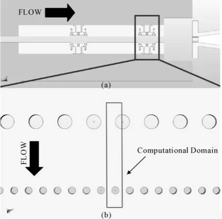
The geometry for the subsonic HICl Laser consists of a rectangular flow channel (Figure 3(a)). There are four rows of secondary flow injection nozzles on the top and bottom plates of the cavity (Figure 3(b)). The primary inlet flow for the subsonic HICl Laser is a mixture of helium (He) and hydrogen (H2). The secondary flow

through the nozzle plates has two different mixtures that are being injected into the primary flow. The first three rows inject a mixture of helium and hydrogen-iodide (HI), where the fourth injects a mixture of helium and nitrogen-trichloride (NCl3). Table 1 shows the boundary

conditions applied during this design optimization run. A constant cross-sectional area was maintained on each inlet, but the aspect ratio was allowed to vary.

It would be computationally expensive to model the entire flow channel for the CFD analysis; consequently, planes of symmetry are used again to reduce the size of

Figure 3. (a) A section view of the laser cavity showing the secondary inlet nozzle plates, and (b) detailed view of one of the nozzle plates. Note: the system has two identical sets of nozzle plates.

Table 1. Flow conditions for subsonic HICl laser.

Initial Conditions and Constants

Pressure 50 torr

Outlet Velocity 83 m/s

Temperature 300 K

Gas Constant 62400 Torr-cm^3/K-mole

the modeled fluid domain (Figure 4). The fluid domain was modeled and meshed using text commands within a journal file. This allowed for easy modification during the automated process.

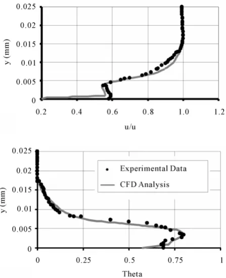
The algorithms, boundary conditions, and meshing strategies for the CFD simulation were validated using experimental data from subsonic (yet compressible flows) jets in cross flow [14]. Downstream velocity and temper-ature profiles obtained from the CFD simulations showed good comparison (Figure 5) to the experimental data of Dizene et al. (2000). This effort highlighted the need to accurately describe the velocity profile at the entrance

Figure 4. Schematic of the variables and geometry for the first probabilistic analysis.

Figure 5. Velocity and Temperature profiles from experi-mental data compared to CFD simulations of jet in cross- flow at X/D = 4.

boundaries and confirmed that the dynamic adaptive grid technique and algorithms selected worked well in these types of fluid flow conditions.

3.2. Probabilistic Model

The initial probabilistic CFD analysis modeled eight geometric variables as distributions. The parameters were the size of the holes in two directions, the offset between the holes, and the hole placement, as illustrated in Figure 4. All of the parameters were modeled as nor-mal distributions defined by mean and standard deviation (Table 2). Standard deviations were determined by the maximum range permissible by geometric limits.

3.3. Optimization Model

Optimization was then applied to determine the values of the variables within the constraints that maximized Mix-edness. The four important variables, LHRx, LHRz, SHRx, and LHRz can be combined into two by keeping the cross sectional areas of the orifices constant. There-fore, only two variables, LHRz and SHRz, need to be perturbed for the HICl Laser optimization. The objective function and constraints for the optimization is stated below:

Maximize: M = f(LHRz, SHRz) (2) Subject to: 0.0055 cm ≤ LHRz ≤ 0.023 cm

0.010 cm ≤ SHRz ≤ 0.042 cm

The optimization routine was used to determine the values of LHRz and SHRz in each analysis. The initial guess in the optimization algorithm were the mean val-ues from the probabilistic analysis. The automated process updated the geometry, generated the mesh, per-formed the CFD analysis and extracted the results to compute the Mixedness parameter. Since the maximum Mixedness is desired, the minimization of the ratio of HI

Table 2. Probabilistic variables with respective mean, stan-dard deviation, and distribution.

Name Mean (mm) StDev (mm) Distribution

LHRx 0.1125 0.067 Normal

LHRz 0.1125 0.067 Normal

SHRx 0.1 0.07 Normal

SHRz 0.1 0.07 Normal

OffsetH 0.2025 0.05 Normal

L_2ndSet 1.5 0.33 Normal

Prcnt1 0.0 0.3 Normal

Prcnt2 0.0 0.3 Normal

concentrations to the maximum concentration (the second term in Equation (1) was calculated. The optimization process continues until the Mixedness value has con-verged to within a 0.01% tolerance. In addition, initial guesses near the lower and upper bounds of the design space were also evaluated to check for local minimums that may be on either side of the mean orifice dimensions.

4. Results and Discussion

4.1. Identification of Important Parameters

Figure 6 shows the importance levels associated with each variable that was perturbed in the modeled geome-try. The importance factors represent the design vector or value of each parameter that defines the MPP, which is proportionate to the output measure at the specified probability. As they are reported in the standard normal space, importance factors are relative measures and the sum of the squares for each measure will equal 1. The importance levels identify the variables that contribute the most to the reliability of the design; therefore, it is deduced from Figure 5 that the radii of the inlet orifices contribute the most to either increase or decrease of the response variable, Mixedness. The other important ob-servation is that PRCNT1, PRCNT2, OFFSETH and L_2NDSET had little to no effect on the Mixedness of the system. Recall, they had the largest standard devia-tion of all the variables. Now, the eliminadevia-tion of four of the eight variables within the geometry allows for the focus on only the radii of the orifices.

4.2. Design Optimization

All of the optimization analyses converged to the same

Figure 6. Histogram of the Importance Levels due to the first probabilistic analysis. It can be seen that the orifices affect the Mixedness the most.

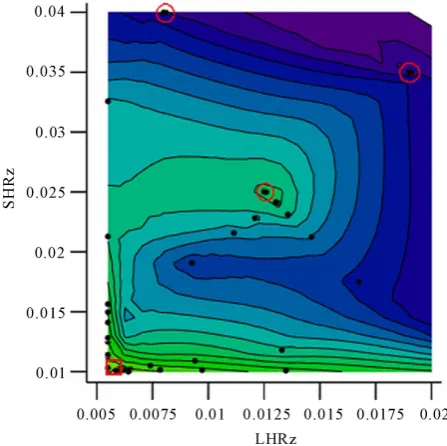
value with the ratio of LHRz to SHRz equal to 0.6. This lower bound is both a computational and manufacturing limit due to the small size of the orifices. Figure 7 shows the contours of all the data taken from the three different optimization runs. The green area shows the larger Mix-edness parameters and the path that the optimization al-gorithm followed. The optimization required between 18 and 29 analyses and from 5 to 9 optimization iterations.

The contour plot of the optimization analysis shows the optimized solution and the various starting points (Figure 8). Since, the only information acquired was along the optimization path, little reliable information can be extracted from the other areas of the plot. This does, however; show the optimal orifice aspect ratio for LHRz and SHRz is approximately equal to 4 and 6, re-spectively, and resulted in an increased Mixedness of nearly 10%. The major diameters of both orifices are parallel to the fluid flow.

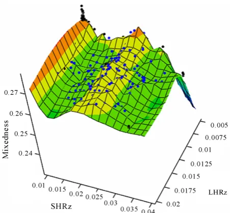
In order to ensure that the global optimum was found, a Monte Carlo simulation was performed using the probabilistic CFD model to characterize the design space used in the optimization analysis. The response surface (Figure 9) with 200 Monte Carlo trials and the optimiza-tion results confirmed the findings of the optimizaoptimiza-tion. Notably, the horizontal bands indicate that the LHRZ dimension has little effect on the fluid system. For ex-ample, starting at the optimized location (SHRz = 0.010 cm, LHRz = 0.006 cm), changes in LHRz within the

Figure 8. Surface plot of the combined Monte Carlo and optimization simulations with data points.

Figure 9. Histograms of the importance levels from the manufacturing sensitivity simulation.

design space did not affect the Mixedness value by more than 1%. Knowledge of these relationships is helpful in the design and manufacturing processes. The LHRz ori-fice can be a simple, circular geometry (which will be easier to create) and the mixing of the system will stay approximately the same compared to if it were elliptical. The response surface is non-monotonic over the optimi-zation design space. The Monte Carlo results also reaf-firm that the optimal configuration of the orifices, where the small orifice is located upstream to large orifice.

4.3. Manufacturing Sensitivities

Based on the optimized design, the probabilistic platform was used to investigate the variability in Mixedness due

to the manufacturing tolerances. The most economical way to create these elliptical geometries at the small di-mensions required is through a wire electrical discharge machine (EDM). In this analysis, the geometry from the optimization simulation with mean values for LHRz and SHRz equal to 0.006 and 0.010 cm, respectively, will be used. The tolerances on these dimensions are +/− 0.001 cm, a tolerance that can typically be achieved by a wire EDM in a cost effective manner. The AMV method in-corporated seven CFD simulations. The values for the AMV simulation are given below in Table 3.

The results for the importance of the four parameters, LHRz, LHRx, SHRz, and SHRz, are show in Figure 1. These results illustrate the same trends as the whole sys-tem. First, the LHRx, LHRz, and SHRx dimensions have virtually no importance on the Mixedness of the system. For the manufacturing design, the relaxation of toler-ances on the LHRz dimensions would reduce the cost of fabrication and still maintaining a high Mixedness num-ber. The importance of SHRz dimension does affect the system and the resulting Mixedness number. This result is liberal because the orifices’ aspect ratios did change slightly. Since the X and Z dimensions were not depen-dent on each other, the X or Z radii could get larger or smaller while the other could do the same. Therefore, the results showed an increase in Mixedness, but if the as-pect ratios were the same the Mixedness should not change. However, the Mixedness number reduces by ~3% if the SHRz dimension is decreased by 0.001 cm and increases by ~3% if it is decreased by 0.001 cm.

5. Conclusions

The purpose of this research was to create and implement an efficient computational design tool to combine opti-mization and probabilistic modeling to provide insight into how to improve chemical mixing systems perfor-mance. This has provided insight into the sensitivities of several different parameters that affect chemical mixing systems. Baseline CFD models were created for subsonic and mixing nozzles. The interfacing tools designed worked with minimal interaction from the user. The au-tomated process for the probabilistic analysis requires

Table 3. Probabilistic variables for manufacturing sensitivi-ties on the optimized orifice geometry.

Name Mean StDev Distribution

LHRZ 0.0060 0.00034 Normal

LHRX 0.0265 0.00034 Normal

SHRz 0.0636 0.00034 Normal

input variables and perturbations from the user (assum-ing the geometry is created). Once all the inputs are spe-cified, the interface carries out numerous evaluations of a fluid system. The optimization interface operated in much the same way. It required a starting point, as well as, constraints on the system. These actions were imple-mented on a subsonic mixing nozzle and results were obtained. Finally, the parallel processing technique enabled complex flows to be optimized in a timeframe consistent with real-time design processes (i.e. less than one week). For the AMV probabilistic analysis with 8 variables, the clock time was approximately 5 hours. The optimization process had a clock time on the order of 3-4 days. All the computations took place on a HP xw8400 Workstation with 2 - 2.33GHz Xeon Quad Core Proces-sors and 4 GB RAM.

It was discovered, using the above computational tools, that in a HICl laser mixing nozzle, elliptical orifices with the major diameter parallel to the flow direction in-creased the mixing within the system by roughly 10%. Haven and Kurosaka (1997) similarly found through experimentation that the injection port geometry had a powerful influence on penetration in the near field [15]. For this case the optimum aspect ratio of the larger ori-fice to be approximately 6 and showed that the small injection orifice should be placed in front of the larger in a staggered alignment pattern.

The second evaluation phase of this work explored the impact of manufacturing tolerances on Mixedness. It was shown that the tolerance on SHRz plays the largest role on mixing quality, and that the shape of the small di-ameter secondary injection orifice does not have a great effect on the Mixedness. In fact, the Mixedness only de-creases by 0.7%

6. Acknowledgments

Financial support for this project was funded by the DOD Joint Technology Office; “Hybrid Iodine Laser Testing,” Contract No. FA8632-05-C-2461.

7. References

[1] S. Peigin and B. Epstein, “Multiconstrained Aerodynamic Design of Business Jet by Cfd Driven Optimization Tool,” Aerospace Science and Technology, Vol. 12, No. 2, 2008, pp. 125-134.

[2] Y. Tahara, D. Peri, E. Campana and F. Stern, “Computa-tional Fluid Dynamics-Based Multiobjective Optimiza-tion of a Surface Combatant Using a Global OptimizaOptimiza-tion

Method,” Journal of Marine Science and Technology, Vol. 13, No. 2, 2008, pp. 95-116.

[3] D. L. Carroll, “Chemical Laser Modeling with Genetic Algorithms,” AIAA Journal, Vol. 34, No. 2, 1996, pp. 338-346.

[4] L. H. Sentman, M. Subbiah and S. W. Zelazny, “Blaze II: A Chemical Laser Simulation Computer Program,” Bell Aerospace Textron, TR H-CR-77-8, 1977.

[5] FLUENT_Inc., FLUENT Documentation, 2006.

[6] A. Haldar and S. Mahadevan, “Probability, Reliability and Statistical Methods in Engineering Design,” John Wiley &Sons, Inc., New York, 2000.

[7] Y.-T. Wu, H. R. Millwater and T. A. Cruse, “Advanced Probabilistic Structural Analysis Method for Implicit Performance Functions,” AIAA Journal, Vol.28, No. 9, 1990, pp. 1663-1669.

[8] S. K. Easley, et al., “Finite Element-Based Probabilistic Analysis Tool for Orthopaedic Applications,” Computer Methods and Programs in Biomedicine, Vol. 85, No. 1, 2007, pp. 32-40.

[9] P. J. Laz, J. Q. Stowe, M. A. Baldwin, A. J. Petrella and P. J. Rullkoetter, “Incorporating Uncertainty in Mechanical Properties for Finite Element-Based Evaluation of Bone Mechanics,” Journal of Biomechanics, Vol. 40, No. 13, 2007, pp. 2831-2836.

[10] J. Nocedal and S. J. Wright, “Numerical Optimization. Springer Series in Operations Research,” Springer-Verlag, New York, 1999.

[11] G. N. Vanderplaats, “Numerical Optimization Tech-niques for Engineers,” Third Edition, Vanderplaats Re-search and Development, Inc., 2001.

[12] R. H. Byrd and R. A. Waltz, “An Active-Set Algorith for Nonlinear Programming Using Parametric Linear Pro-gramming,” Department of Industrial and Systems Engi-neering, University of Southern California, Los Angeles, 2007.

[13] MATLAB, The MathWorks Inc., 1994-2008

[14] R. Dizene, J. M. Charbonnier, E. Dorignac and R. Leblanc, “Experimental Study of Inclined Jets Cross Flow Interaction in Compressible Regime. I. Effect of Compressibility in Subsonic Regime on Velocity and Temperature Fields,” International Journal of Thermal Sciences, Vol. 39, No. 3, 2000, pp. 390-403.

[15] B. A. Haven and M. Kurosaka, “Kidney and Anti-Kidney Vortices in Crossflow Jets,” Journal of Fluid Mechanics, Vol. 352, No. , 1997, pp. 27-64.

Nomenclature

L_2ndSet = length to second set of orifices LHRx = first orifice x-direction’s radius LHRz = first orifice z-direction’s radius

Mf = mole fraction

Mf_Homogeneous = homogeneous mole fraction across down-stream plane

N = number of nodes

OffsetH = Distance between first and second orifices within each set

Prcnt1,2 = percent offset between centers of first and second orifices