Computational Optimization of Manufacturing Batch Size and Shipment for an Integrated EPQ Model with Scrap

Computational Optimization of Manufacturing Batch

Size and Shipment for an Integrated EPQ

Model with Scrap

Yuan-Shyi Peter Chiu1, Hong-Dar Lin1, Ming-Hon Hwang2*, Nong Pan3

1_{Department of Industrial Engineering & Management, Chaoyang University of Technology, Taichung, Chinese Taipei} 2_{Department of Marketing and Logistics Management, Chaoyang University of Technology, Taichung, Chinese Taipei}

3_{Department of Business Administration, Chaoyang University of Technology, Taichung, Chinese Taipei}

E-mail: *_{[email protected]}

Received March 12, 2011; revised April 2, 2011; accepted April 28, 2011

Abstract

This paper employs mathematical modeling and algebraic approach to derive the optimal manufacturing batch size and number of shipment for a vendor-buyer integrated economic production quantity (EPQ) model with scrap. Unlike the conventional method by using differential calculus to determine replenishment lot size and optimal number of shipments for such an integrated system, this paper proposes a straightforward alge-braic approach to replace the use of calculus on the total cost function for solving the optimal production- shipment policies. A simpler form for computing long-run average cost for such a vendor-buyer integrated EPQ problem is also provided.

Keywords:Computational Optimization, Manufacturing Batch Size, Shipments, EPQ Model, Random Scrap Rate, Algebraic Approach

1. Introduction

The economic production quantity (EPQ) model was first introduced by Taft [1] to assist practitioners in produc-tion and inventory control field to determine the economic replenishment batch size that minimizes total produc-tion-inventory costs. Classic economic production quan-tity model assumes a continuous inventory issuing policy for satisfying customer’s demand. However, in real world vendor- buyer system, multiple or periodic deliv-eries of finished products are often adopted. Therefore, “how many shipments should a manufacturing lot be broken down to?” becomes another critical issue that practitioners must address in order to minimize overall production-inventory-delivery costs.

Studies related to various aspects of supply chain op-timization have been extensively carried out (see for ex- ample [2-9]) in past decades. Goyal [2] examined an integrated single supplier-single customer problem. He proposed a method that is typically applicable to those inventory problems where a product is procured by a single customer from a single supplier. Example was provided to demonstrate his proposed model. Schwarz et

Y.-S. P. CHIU ET AL. ₂₀₃ ordering policy for raw materials as well as the

manu-facturing batch size, so that the overall costs for such a supply chain system can be minimized. Chiu et al. [9] incorporated a multi-delivery policy and quality assur-ance into an imperfect economic production quantity (EPQ) model with scrap and rework. They assumed that the random defective items produced are partially re-pairable and are reworked in each cycle when regular production ends, and the finished items can only be de-livered to customers if the whole lot is quality assured at the end of rework. Fixed quantity multiple installments of the finished batch are delivered to customers at a fixed interval of time. The expected integrated cost function per unit time was derived. A closed-form optimal batch size solution to the problem was obtained.

Imperfect quality items produced in real world manu-facturing environments is another inevitable and impor-tant issue that practitioners in the production manage-ment filed must deal with. In the past decades, many studies have been carried out to address the issue of de-fective items in the production lines (see for example [10-14]). The nonconforming items sometimes can be repaired through rework, hence overall production costs can be significantly reduced [15-20]. Yu and Bricker [15] presented an informative application of Markov Chain analysis to a multistage manufacturing problem. Jamal et al. [16] studied the optimal manufacturing batch size with rework process at a single-stage production system. Cases of rework being completed within the same pro-duction cycle, and rework being done after N cycles are examined. They developed mathematical models for each case and derived total system costs and optimal batch sizes accordingly. Chiu et al. [19] proposed a nu-merical method for expediting scrap-or-rework decision making in EPQ model with failure in repair.

Algebraic approach for determining economic order quantity (EOQ) model with backlogging was introduced by Grubbström and Erdem [21]. They proposed algebraic derivations to solve the optimal order quantity without reference to the first-order or second-order differentia-tions. Various aspects of supply chain optimization stud-ies have employed the same or similar methodologstud-ies [22,23]. This paper uses mathematical modeling to de-rive the long-run average cost function for the proposed vendor-buyer integrated EPQ model with scrap; then employs such a straightforward algebraic derivation to determine the optimal production-shipment policies for the proposed EPQ model.

2. The Proposed Model and Mathematical

Modeling

The proposed economic production quantity model

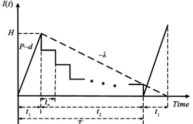
as-sumes there is an x portion of defective items produced randomly at a production rate d during regular produc-tion time. All produced items are screened and inspecproduc-tion cost per item is included in the unit production cost C. All nonconforming items are assumed to be scrap and will be discarded at the end of production. Under regular supply (not allowing shortages), the constant production rate P must be larger than the sum of demand rate λ and production rate of scrap items d. That is: (P – d – λ) > 0. The production rate of scrap items d can be expressed as d = Px.

A multi-delivery policy is considered in this study and it is also assumed that the finished items can only be de-livered to customers if the whole lot is quality assured at the end of production process. Fixed-quantity n install-ments of finished batch are delivered to customers at a fixed interval of time during the production downtime t2

(see Figure 1). Additional notation is listed in Nomen-clature in Appendix.

TC(Q, n), the total production-inventory-delivery costs per cycle consists of 1) setup cost; 2) variable production costs; 3) variable scrap disposal costs; 4) fixed delivery cost; 5) variable delivery costs; 6) variable holding costs at the supplier side for all items produced (defective and perfect quality items) in t1 and all items waiting to be

delivered in t2; and 7) holding cost for finished goods

stocked at customer’s end. Therefore, TC(Q, n) is





 





 





1 1

1 2

2

2 2

,

1

1

2 2

2

S T

TC Q n

K CQ C xQ nK C Q x

H dt n

h t Ht

n

h H

t T H t

n 

     _  _ 

    

 _{    }

 

 

 

 _   _

 

[image:2.595.335.540.409.501.2]

(1)

Figure 2 shows supplier’s inventory holding during delivery time t2. The variable holding costs for finished

products kept by the supplier in delivery time t2 are

[image:2.595.327.521.557.682.2]

1) When n = 1, total holding cost in delivery time = 0. 2) When n = 2, total holding costs in delivery time be- come (see Figure 2)

2

2 2

1

2 2 2

t H

h_  _{  }h 

 

  Ht (2) 3) When n = 3, total holding costs in delivery time are

2 2 2 2 2 1 3 3 t t H H

h_    _{ }h _

    

  Ht (3) 4) When n = 4, total holding costs in delivery time be- come

2 2 2

2 2

4 4 4 4

t t t

H H H

h_      __{ }h  _

     

  Ht (4)

Therefore, the following general term for total holding costs during t2 can be obtained (as shown in Equation (1)

above):

1

2 2

2 2

1

1 1 ( 1)

2 2

n i

n n n

h i Ht h Ht h Ht

n n n         _     _          

 



       2

1

(5) Taking randomness of scrap rate into consideration and employing the expected values of it, and with further derivations, the long-run average costs per unit time for the proposed EPQ model, E[TCU(Q, n)] can be derived as follows (refer to a similar derivation procedure in [9]):









 

 





 







 

 



 







 



 





1 2 , ,

1 1 1

1 1 2 2 2 1 1 1 1 2 S T

E TCU Q n E TC Q n

E T

C E x K nK

C

C

E x Q E x E x

hQ E x

hQ n hQ

n P

P E x

h Q n

E x

n n P

   _                            _{ }      _ _        _{ }  _{  }       (6)

3. Deriving Optimal Production-Shipment

Policies without Derivatives

This study employs algebraic approach to derive the op-timal production-shipment policies, instead of using dif-ferential calculus on E[TCU(Q, n)] with the need of prov-ing its optimality [21-23]. In Equation (6), both Q and n are decision variables, by rearranging terms in Equation (6) as the constants, Q–1_{, Q, nQ}–1_{, and Qn}–1

, one has





 

 







1

1 2 3

1

4 5

,

E TCU Q n Q Q

nQ n Q

[image:3.595.313.536.81.204.2]

                

Figure 2. On-hand inventory of the finished items kept by supplier during t2 in the proposed EPQ model.

where β1, β2, β3, β4, and β5 denote the following:

 



 

 



1

1 1

S

T

C E x

C _C

E x E x

 

    

  (8)

 







 







2 2 1 2 2 2 1

h E x

h

h h P

P E x

               (9)

 





3 1 K E x    

 (10)

 



1



4 1 K E x    

 (11)

 





_

5 2 1 2 2 E x h h P        



        (12)

With further rearrangements, Equation (7) becomes







 



1 2 3

4 5 1 2 2 1 1 ,

E TCU Q n Q Q

n Q nQ

                       _  _   (13)









  

 

 







  







 

 





1 2 3 2 3

4 5 4 5

2 3 4 5

2 2 ` 2 2 1 1 1 1 , 2 2 2 2

E TCU Q n

Q Q Q

n Q nQ nQ

Q Q n Q nQ

                          _     _   1 1      _   _        _  _ _{ } (14)

















1 2 4 5

2 3 4 5

2 1 2 1 1 , 2 2

E TCU Q n Q Q

n Q nQ

                      _{ }    _  _     3 (15)



Y.-S. P. CHIU ET AL. ₂₀₅



* *



1 2 3 4

, 2 2

E TCU Q n It is noted that if the following square terms

(Equa-tions (17) and (18)) equal zero, then Equation (15) will be minimized:

5

    

 _{  }   

  (22)

4. Demonstrative Example





2 1

2 3 0

Q _  Q   _  (16)

Consider a product can be produced at an annual rate of 60,000 units and this item has experienced a flat demand rate of 3,400 units per year. Assume that during produc-tion process a random scrap rate which follows a uniform distribution over the interval [0, 0.3]. In additions, the following values of related variables are considered:









2

1 1

4 5 0

n Q  nQ  _   _

  (17) or

* 3

2

Q 



 (18)

C = $100 per item, and

CS = $20, disposal cost per scrap item,

* 5 4

*

n 



 Q (19) h = $20 per item per year,

h2 = $80 per item kept at the customer’s end per unit

time, Substituting Equations (9) and (10) in Equation (18),

the optimal replenishment lot size Q* _{can be obtains: K = $20,000 per production run,} K1 = $4350 per shipment, a fixed cost,

 











 



*

2

2

2 1

K Q

h _{h E x h h E x}

P P



 



    1

(20) CT = $0.1 per item delivered.

Substituting Equations (11), (12), and (20) in Equation (19), the optimal number of shipments is







 





 



 











 



2

2 1

1 1

*

1 1

K h h E x E x

P n

h

K h E x h h E x

P P



 



  _  



 _{    }



 2

 

  

From Equations (21), one obtains the optimal number of delivery n* _{= 3. By plugging n}*

back into Equation (7) and resolving the algebraic solution for Q*

one finds the optimal production batch size Q*

= 2652. Calculating Equation (22) one obtains the long-run average cost E × [TCU(Q*_{, n}*

)] = $512,047. Figure 3 shows the convexity of the long-run integrated cost function E[TCU(Q, n* ₌ 3)].

It is noted that n*

should practically be an integer nu- mber, but Equation (21) gives a real number. In order to obtain the optimal integer value of n, one should com-pute the E[TCU(Q, n)] for both integers that are adjacent to real number n*

respectively (for instance, in this ex-ample Equation (21) gives n* _{= 3.1733, so both n = 3 and} n = 4 must be plugged in E[TCU(Q, n)]), and select the one with minimum cost as our optimal n*

. (21)

One notes that Equation (21) is identical to what was obtained by using the conventional differential calculus method on E[TCU(Q, n)] [24]. Further, from Equation (7) the optimal cost function E[TCU(Q*_{, n}*

[image:4.595.155.445.518.704.2]

)] is

5. Conclusions

This paper derives the optimal manufacturing batch size and number of shipment for a vendor-buyer integrated EPQ model with scrap using mathematical modeling and algebraic approach. It is confirmed the research results from the proposed algebraic derivations are identical to what were derived by the use of conventional differential calculus. In additions, this study also reveals a simpler computation formula (i.e. Equation (22)) for the long-run average cost function for such a vendor-buyer integrated EPQ problem. This straightforward algebraic approach enables practitioners or students who with little or no knowledge of calculus to learn or handle with ease the real-life EPQ model.

6. Acknowledgements

The authors greatly appreciate the National Science Coun- cil of Taiwan for supporting this research under grant number: NSC 99-2221-E-324-017.

7. References

[1] E. W. Taft, “The Most Economical Production Lot,” Iron

Age, Vol. 101, 1918, pp. 1410-1412.

[2] S. K. Goyal, “Integrated Inventory Model for a Single Supplier-Single Customer Problem,” International

Jour-nal of Production Research, Vol. 15, No. 1, 1977, pp. 107-111.

[3] L. B. Schwarz, B. L. Deuermeyer and R. D. Badinelli, “Fill-Rate Optimization in a One-Warehouse N-Identical Retailer Distribution System,” Management Science, Vol. 31, No. 4, 1985, pp. 488-498.

[4] L. Lu, “A One-Vendor Multi-Buyer Integrated Inventory Model,” European Journal of Operational Research, Vol. 81, No. 2, 1995, pp. 312-323.

[5] R. A. Sarker and L. R. Khan, “Optimal Batch Size for a Production System Operating under Periodic Delivery Policy,” Computers and Industrial Engineering, Vol. 37, No. 4, 1999, pp. 711-730.

[6] S. Viswanathan and R. Piplani, “Coordinating Supply Chain Inventories through Common Replenishment Ep-ochs,” European Journal of Operational Research, Vol. 129, No. 2, 2001, pp. 277-286.

[7] M. Eben-Chaime, “The Effect of Discreteness in Vendor- Buyer Relationships,” IIE Transactions, Vol. 36, No. 6, 2004, pp. 583-589.

[8] R. M. Hill and M. Omar, “Another Look at the Single- Vendor Single-Buyer Integrated Production-Inventory Problem,” International Journal of Production Research, Vol. 44, No. 4, 2006, pp. 791-800.

[9] Y.-S. P. Chiu, S. W. Chiu, C.-Y. Li, and C.-K. Ting, “In-corporating Multi-Delivery Policy and Quality Assurance into Economic Production Lot Size Problem,” Journal of

Scientific & Industrial Research, Vol. 68, No. 6, 2009, pp. 505-512.

[10] M. J. Rosenblatt and H. L. Lee, “Economic Production Cycles with Imperfect Production Processes,” IIE

Trans-actions, Vol. 18, No. 1, 1986, pp. 48-55.

[11] K. Moinzadeh and P. Aggarwal, “Analysis of a Produc-tion/Inventory System Subject to Random Disruptions,”

Management Science, Vol. 43, No. 11, 1997, pp. 1577- 1588.

[12] A. Chelbi and N. Rezg, “Analysis of a Production/In- Ventory System with Randomly Failing Production Unit Subjected to a Minimum Required Availability Level,”

International Journal of Production Economics, Vol. 99, 2006, pp. 131-143.

[13] S. W. Chiu, Y.-S. P. Chiu and C.-C. Shih, “Determining Expedited Time and Cost of the End Product with Defec-tive Component Parts Using Critical Path Method (CPM) and Time-Costing Method,” Journal of Scientific &

In-dustrial Research, Vol. 65, No. 9, 2006, pp. 695-701. [14] J. Li, D. E. Blumenfeld and S. P. Marin, “Production

System Design for Quality Robustness,” IIE Transactions, Vol. 40, No. 3, 2008, pp. 162-176.

[15] K-Y. C. Yu and D. L. Bricker, “Analysis of a Markov Chain Model of a Multistage Manufacturing System with Inspection, Rejection, and Rework,” IIE Transactions, Vol. 25, No. 1, 1993, pp. 109-112.

[16] A. M. M. Jamal, B. R. Sarker and S. Mondal, “Optimal Manufacturing Batch Size with Rework Process at a Sin-gle-Stage Production System,” Computers & Industrial

Engineering, Vol. 47, No. 2, 2004, pp. 77-89.

[17] S. W. Chiu and Y.-S. P. Chiu, “Mathematical Modeling for Production System with Backlogging and Failure in Repair,” Journal of Scientific & Industrial Research, Vol. 65, 2006, pp. 499-506.

[18] S. W. Chiu, “Production Run Time Problem with Ma-chine Breakdowns under AR Control Policy and Re-work,” Journal of Scientific & Industrial Research, Vol. 66, No. 12, 2007, pp. 979-988

[19] S. W. Chiu, K.-K. Chen and H.-H. Chang, “Mathematical Method for Expediting Scrap-or-Rework Decision Mak-ing in EPQ Model with Failure in Repair,” Mathematical

and Computational Applications, Vol. 13, No. 3, 2008, pp. 137-145.

[20] S. W. Chiu, “Robust Planning in Optimization for Pro-duction System Subject to Random Machine Breakdown and Failure in Rework,” Computers & Operations

Re-search, Vol. 37, No. 5, 2010, pp. 899-908.

[21] R. W. Grubbström and A. Erdem, “The EOQ with Back-logging Derived without Derivatives,” International

Journal of Production Economics, Vol. 59, No. 1-3, 1999, pp. 529-530.

[22] S. W. Chiu, “Production Lot Size Problem with Failure in Repair and Backlogging Derived without Derivatives,”

European Journal of Operational Research, Vol. 188, No. 2, 2008, pp. 610-615.

Y.-S. P. CHIU ET AL. ₂₀₇ for EPQ Model with Rework Process,” Mathematical and

Computational Applications, Vol. 2010, No. 3, 2010, pp. 364-370.

[24] S. W. Chiu, H.-D. Lin, C.-B. Cheng and C.-L. Chung,

“Optimal Production-Shipment Decisions for the Finite Production Rate Model with Scrap,” International

Jour-nal for Engineering Modelling, Vol. 22, Issues 1-4, 2009, pp. 15-24.

Appendix

Nomenclature:

C = unit manufacturing cost, CS = the disposal cost per scrap item,

h = unit holding cost,

K = setup cost per production run, K1 = fixed delivery cost per shipment,

CT= unit delivery cost CT,

Q = production lot size, a decision variable, to be de-termined for each cycle,

T = production cycle length,

n = number of fixed quantity installments of the fin-ished batch to be delivered to customers, a decision vari-able, to be determined for each cycle,

d = production rate of scrap items,

t1 = the production uptime for the proposed EPQ

model,

t2 = time required for delivering all finished products,

H = maximum level of on-hand inventory in units when regular production process ends,

tn = a fixed interval of time between each installment

of finished products delivered during production down-time t2,

I(t) = on-hand inventory of perfect quality items at time t,

TC(Q, n) = total production-inventory-delivery costs per cycle for the proposed model,