Communications and Network, 2010, 2, 235-245
doi:10.4236/cn.2010.24034 Published Online November 2010 (http://www.SciRP.org/journal/cn)
All-Optical Cryptographic Device for Secure
Communication
Fabio Garzia, Roberto Cusani
INFOCOM Department, SAPIENZA – University of Rome, Rome, Italy E-mail: [email protected]
Received March 3, 2010; revised May 7, 2010; accepted April 23, 2010
Abstract
An all-optical cryptographic device for secure communication, based on the properties of soliton beams, is presented. It can encode a given bit stream of optical pulses, changing their phase and their amplitude as a function of an encryption serial key that merge with the data stream, generating a ciphered stream. The greatest advantage of the device is real-time encrypting – data can be transmitted at the original speed with-out slowing down.
Keywords:Cryptographic Device, Security Device, Soliton Interaction, All-optical Switching, Spatial Soli-ton, All-optical Device.
1. Introduction
The device described in this paper is capable of codify-ing a given bit stream of optical pulses, changcodify-ing their phase and their amplitude as a function of an encryption serial key that merges with the data stream, generating a ciphered stream. It is based on the special properties of spatial solitons that are, as well known, self-trapped op-tical beams able to propagate without any change of their spatial shape, thanks to the equilibrium, in a self-focus-ing medium, between diffraction and nonlinear refraction [1].
Their interesting properties have allowed to design a certain number of spatial optical switches which utilize the interaction between two bright or dark soliton beams, and the waveguide structures induced by these interac-tions [2-6]. Two distinct parallel solitons are generally used as initial condition for such interactions. In fact it is well known that when two distinct bright spatial solitons are launched parallel to each other, the interaction force between them depends on their relative distance and their phase [7,8].
A variety of useful devices can be thought and de-signed using the properties of solitons. One of the most important features is their particle-like behaviour and their relative robustness to external disturbs.
Interesting effects have been found in the study of transverse effects of soliton propagation at the interface between two nonlinear materials [9-11] or in a material
in the presence of a Gaussian refractive index profile, that is in low perturbation regime [12].
It has been shown that it is possible to switch a soliton, in the presence of a transverse refractive index variation, towards a fixed path, since the index variation acts as a perturbation against which the soliton reacts as a particle, moving as a packet without any loss of energy. This last property makes possible to design useful all optical de-vices such as a filter [13] or a high speed router [14], thanks to the possibility of generating spatial soliton in real material [15-17].
The general problem of encrypting the data transmit-ted on an optical medium is very felt in the security field [18-33].
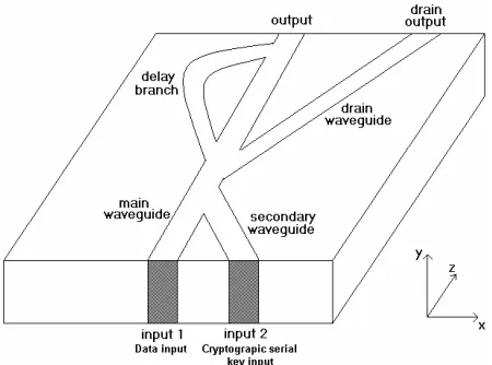
The aim of the present work is to find a new approach to this problem, studying a device that is able to increase the security level of an optical channel, extending the modulation also to the phase of the output pulses. It acts as an amplitude/phase converter accepting two binary modulated stream of pulses as inputs and generating a unique phase modulated stream of pulses as output. The first stream is related to the data stream while the second stream is related to the serial cryptographic key. The great advantage is that the device is totally passive, which means that is does not need extra energy to work properly. The working principle is shown in Figure 1.
In its basic geometry a soliton beam travels in a waveguide which, in the plane between the cladding and
F. GARZIA ET AL.
[image:2.595.141.455.75.208.2]236
Figure 1. Working principle of the device.
follows a triangular curve, with a modified parabolic profile.
We start studying the general structure of the device. Then the transverse behaviour of a soliton in a triangular profile [13], whose longitudinal profile is parabolic [14], is discussed. Once the properties of motion are derived, we investigate the structure from the global point of view, deriving all the properties and the operative conditions, that represents the scope of this paper.
2. Structure of the Device
To simplify the development of the theory we consider only a 2-in-1-out device. The function of the device is to generate a phase modulated pulse according to the dif-ferent combinations of amplitude of input pulses, that represent the data stream and the cryptographic stream. In the following we briefly call them input 1 and input 2. This is equal to say that, in the presence of two binary inputs, the possible amplitude combinations are 4, and the output pulse has to assume 4 different phase values, without requesting auxiliary energy.
We suppose to work with soliton beams to use their attracting or repelling properties [7] and their particular behaviour when they propagate in a transverse refractive index profile [13]. The structure we want to study is shown in Figure 2.
We also suppose that the two input pulses enter in the relative inputs of the device with the same phase. This is not a restriction since any phase difference can be prop-erly compensated.
Owed to the fact that we deal with equal streams of pulses the last condition means that the input pulses are characterised by the same amplitude.
The device is composed by 4 parts: the main waveguide, the secondary waveguide, the delay branch and the drain waveguide. The geometry and the refrac-tive index values of these four components strictly de-termine the features of the device and their values will be designed as discussed in the following.
Let us analyse the behaviour of the device in the four possible input situations. Since we deal with binary input pulses we consider the two values of logical zero (ab-sence of pulse) and logical one (pre(ab-sence of pulse). We refer to them as zero and one.
The first situation is when the two inputs are equal to zero. In this case, due to the passive nature of the device, we obtain a zero in the output.
The second situation is when the first input is equal to one and the second input is equal to zero. In this case, if the refractive index of both the delay branch and the drain waveguide is less or equal to the refractive index of the main waveguide, the pulse propagates undisturbed and it reaches the output, with a phase that is equal to the propa-gation phase along the main waveguide. If the length of this waveguide is properly chosen, according to the wave-length of the beam, the phase of the output pulse is equal to the phase of the input pulse. In the first situation there was an absence of pulse and its phase value was virtually equal to zero. In this case the phase value variation has been chosen equal to zero but we are in the presence of a pulse. The phase variation could anyway be chosen at will, but we keep it fixed at zero for simplicity. The behaviour of this kind of waveguide has already been studied [13].
[image:2.595.308.533.531.698.2]237
The third situation is when the first input is equal to zero and the second input is equal to one. In this case, since we are in the proper refractive index conditions of the waveguide and the delay branch is properly shifted with respect to the input point of the secondary wave, the second input pulse is trapped in the main waveguide and it reaches the output with a certain phase difference, that we define later, with respect to the previous case due to the fact that it propagates, in the initial part, into the secondary waveguide.
The fourth situation is when both the inputs are equal to one. In this case the two pulses meet at the converging point between the main waveguide and the secondary waveguide. In this case, since we are in soliton propaga-tion condipropaga-tion, they can attract if their relative phase is included between zero and /2 or between 3/2 and 2, or they can repel if their relative phase is included be-tween /2 and 3/2. If the length of the secondary waveguide is chosen to generate a repulsive condition, the two solitons propagate in the main waveguide prop-erly separated until reaching the bifurcation point be-tween the main waveguide, the delay branch and the drain waveguide. At this point the two solitons detach: the first one enters the delay branch while the second one enters the drain waveguide.
The first soliton propagates in the delay branch ex-periencing a phase variation that depends on the length of the branch and therefore is properly selectable and can be chosen different from the previous cases, generating the fourth phase condition. The second pulse, on the contrary, propagates in the drain waveguide where it reaches the proper drain output.
The delay branch is composed by a properly modified longitudinal parabolic waveguide, whose purpose is to accept the beam from the main waveguide with an angle that respects the paraxial approximation, to propagate it changing its direction until reaching a straight longitudi-nal direction and to reverse this sequence until carrying the pulse inside the main waveguide with a certain phase difference. The behaviour of this modified parabolic waveguide is studied later.
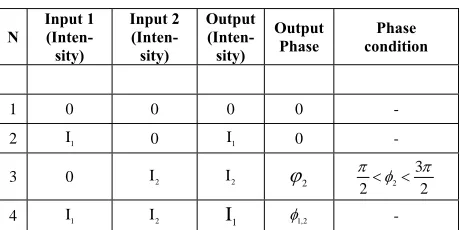
The situation is summarised in Table 1, where it is also pointed out the pulse that reaches the output to pro-vide more details about the working principles of the device, even if we consider input pulses with the same amplitude.
3. Properties of a Soliton in a Modified
Longitudinal Parabolic Waveguide
[image:3.595.309.539.91.206.2]We want now to define the structure of the modified parabolic waveguide composing the delay branch to find its peculiar properties that allow the loop to work prop-erly.
Table 1. Working scheme of the device.
N
Input 1
(Inten-sity)
Input 2
(Inten-sity)
Output
(Inten-sity)
Output
Phase condition Phase
1 0 0 0 0 -
2 I 1 0 I 1 0 -
3 0 I2 I2 2 2
3
2 2
4 I1 I2 I1 1,2 -
We choose this kind of waveguide because it is the simplest curve that carries progressively the soliton beam from a propagation angle that respects the paraxial ap-proximation until an angle that respects a parallel longi-tudinal propagation and vice versa.
This curve could be roughly approximated with a lin-ear curve, but the final result would be a too sharp path, since the soliton reaches the reversing point with a cer-tain inclination. Further the parabolic path is the trajec-tory followed from a soliton beam that is injected into a linear transverse refractive index profile, that is the transverse profile that we are going to consider.
Let us consider a soliton beam propagating in the z-direction, whose expression of the field Q at the begin-ning of the structure is:
x,0 Csech
C
x-x
Q
(1) where x is the position of the centre of the beam and C is a real constant from which both the width and the amplitude of the field depend. The variables x and z are normalised with respect to the wavevector of the wave and therefore they are adimensional quantities.
When the soliton beam is propagating in a triangular transverse index profile, whose maximum value is n0
and whose maximum width is 2b, it is subjected to a transverse acceleration equal to [13,14]:
2 0
2
T
n a
b
C (2)
We use, for our analysis, a dynamic point of view, that is to consider the step by step transverse relative position of the waveguide with respect to the beam using the z variable as a time parameter.
If xG
z is the position of the central part of thewaveguide profile with respect to z, the longitudinal form of the waveguide is chosen to be a modified parabolic:
222
G
z d
x z
a a
z (3)
238 F. GARZIA ET AL.
the position of the curve. Equation (3) can be better un-derstood if it is expressed as a function of z, that is:
G
z a x d a d (4) It is possible to see that it is positioned in the second quadrant of the Cartesian plane, it has a vertical asymp-tote at xG
z d when za d. It shows agradu-ally increasing derivative, growing from a starting angle at x=0, chosen to be below the maximum angle allowed from the paraxial approximation, until reaching a vertical alignment at xG
z d, that is what we want to makethe device work properly. To respect this term it is nec-essary to impose a certain condition to the ‘a’ and ‘d’ parameters, as we show later. A graphical representation of (4) is shown in Figure 4 for a=16.9 and d=1.4.
The local inclination of the waveguide with respect to the longitudinal axis z, can be regarded as the transverse relative velocity of the waveguide that appears to the beam that propagates longitudinally:
2
2 2
vG G
dx z z
dz a a
d (5)
Using (2) it is possible to calculate the transverse rela-tive velocity:
2 0
0
2 v
z
B T
n
a d C z
b
(6)and the position of the beam
2 2 0
0
v
z
B B
n
x d C
b
z (7) [image:4.595.321.530.467.693.2]Equation (7) is valid for a propagation in the first quadrant of Cartesian plane. Since we consider, in our case, a propagation in the second quadrant, we must re-verse the sign of the second member of the equation con-sidered.
Figure 4. Graphical representation of the modified para-bolic waveguide for a=16.9, d=1.4, in normalized units.
Initially the beam is positioned in the centre of the waveguide. Since the waveguide appears to move, with respect to an observer that follows the longitudinal direc-tion, with a relative velocity expressed by (5), the soliton beam enters in the constant acceleration zone, where its velocity increases linearly with z. It also follows a para-bolic trajectory, according to (7), until it remains in this part of the waveguide.
After that the beam has propagated for a certain z dis-tance, two different situations may happen: the beam leaves the acceleration zone without reaching the veloc-ity of the waveguide at that z, or the beam acquires a velocity that is greater than or equal to the velocity of the waveguide. The first event may called ‘detach situation’, since the beam leaves the waveguide, while the second one may be called ‘lock-in situation’ since the beam reaches the other side of the waveguide where it is stopped, reversing its path and so on.
At any value of z, as shown in Figure 3, the distance
BG
d between the beam and the waveguide is:
2 2
2 0
2
2 2
2 0
2
2
2
BG B G
n C z d
d x x z
b a a
b a n C d
z z
a a b
z
b
(8)
A detach situation takes place when:
BG
d (9) If we solve (9) with respect to z, we can calculate, if it exists, the propagation distance where the detachment begins:
2 2
0
2 2
0 D
d d b a n C z
b a n C ab
(10)
[image:4.595.69.273.529.690.2]239
The two solutions refer to the detach situation (when the negative sign of the root is considered) or to the first cross of the centre of the waveguide in the lock-in situa-tion (when the positive sign of the root is considered). Studying the discriminator of (10) it is possible to derive the value of the amplitude CD that divides the lock-in
values from the detach values: 1 2
0 1
D
d b
C
a n
(11)
It is possible to see, from (11), that the more the cur-vature of the waveguide (‘a’ parameter) increases or the more the refractive index decreases and the more CD
increase. This behaviour agrees with what one could ex-pect.
We want now to calculate the inclination according to which a soliton, whose amplitude is smaller than the de-tach amplitude, leaves the waveguide. Since the men-tioned angle is equal to the detach velocity, substituting (11) into (6), we have:
1 tan vD
(12a)
and
0 22 2
0
2
vD vB zD n C a (
b a n C
d
2 2
0 )
d b a n C
(12b)
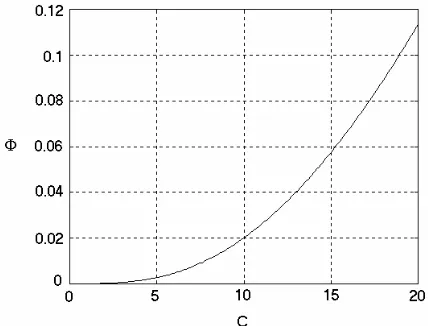
In Figure 5 it is shown the graphical behaviour of (12) for a=16.9, d=1.4, b=0.25, . The detach value
5 0 1 10
n
D
C can be calculated by means of (11) and it is equal to 20.
Due to the absence of restrictions about the length L of the waveguide, the lock-in value CD of the amplitude,
expressed from (11), does not depend on L. This means that, given a certain waveguide whose length is equal to L, we can obtain a lock-in value CD whose detachment
distance, calculated from (10), is longer than L. In this situation, due to the restriction imposed from the waveguide length L, the detach value CD obviously
decreases. In fact, even if the beams characterised from an amplitude lesser thanCD tend to be expelled from the
waveguide, the detachment takes place at a distance that is longer than the waveguide length L and the beam re-mains locked-in. The new value CD, that is lower than
D
C , can be calculated from (10) setting zDL and
solving respect to C:
2 4
2
DL
B B AC
C
A
(13a)
where
4 2 2 0
A a n L (13b)
2 2 3 4 2
0 0
2 2
B a bL n a b d L n a b n0 (13c)
2 2 2 2 3
2
Cb L ab L da b (13d) We want now to make some considerations about the paraxial approximation.
Since we deal with a modified parabolic waveguide, we are in the presence of a curvature, with respect to the z axis, that increases with z. We have not to forget that we are in a paraxial approximation, that is the derived equations are valid until the angle between the propaga-tion direcpropaga-tion and the longitudinal direcpropaga-tion is lesser than 8°10°. This means that, due to the analytical expression of the waveguide, expressed from (3) or (4), once the ‘a’ or ‘d’ parameter has been chosen the other parameter is unavoidably fixed. The condition must be imposed only at the entrance of the waveguide, where the curvature, with respect to the longitudinal direction is maximum and decreases up to zero at the end. In analytical terms this means that it is possible to impose this condition to the first derivative of (3) to calculate the maximum propagation distance:
20 tan 8
G
d x
a
0,14 (14)
that gives:
2
7 10
d a
(15)
This condition must be considered in the project of the delay branch.
We want now to calculate the length of the curve ex-pressed by (3), since it is necessary to control the optical path, and therefore the phase variation, of the beam that propagates inside it.
[image:5.595.316.530.530.693.2]Considering (4), the first derivative of z with respect to x is:
240 F. GARZIA ET AL.
2
dz a
dx xd (16)
and the elementary length of the curve, as a function of x is:
2
2 2 2
4
a
dl dx dz dx dx
x d
2
(17)
Integrating (17) we have:
2 2 4 4 log(8 8 2 8x d a
x d a x d I x
x d
22 4 4x 4d a ) constant
a x d
x d
(18)
It is possible to see that the integral becomes indefinite when x tends to -d, as one could expect due to the struc-ture of the curve. To define the constant that is present in Equation (18) it is necessary to calculate the limit of the integral when x tends to -d:
2lim log
4
x d
a I x
a (19)
The length of the curve is therefore equal to:
2 2
22 2 2
4
0 log
2 8
4 4
4 ) 4 ) l
4
G
d d a a
L I d a
d
d a d a a
d d d d 8 oga (20)
that is obviously a complex function of ‘a’ and ‘d’ pa-rameters.
4. Numerical Simulation of the Effect
We have simulated the device from the numerical point of view using a FD-BPM algorithm to study its behav-iour and to see if it agrees with the developed theory.
At first the design does not consider the physical limi-tations that can arise when we deal with technological fabrication problems. In the next paragraph we will con-sider this kind of problems.
We use, in this situation, a geometrical approach, that is we do not care of imposing particular conditions that would be necessary in a real situation, such us to use the same 0 for all the waveguides, letting us a higher
number of degrees of freedom. We are further free of using the wavelength we need to generate the proper phase variation according to our needs. This is not obvi-ously possible in a real case where the wavelength is given.
n
Let us choose for example the half length of the delay
branch waveguide equal to 20: 20
a d (21) Since we have to respect, even in this design approach, the paraxial condition, we have to solve the system of equations composed by (21) and (15) that gives a = 16.9, d=1.4.
The width of the waveguide must obviously be less than ‘d’ and we choose, for example b = 0.25, that is to suppose a waveguide width equal to 2b = 0.5.
The spot size of the beam must be less or equal to ‘b’. Since we deal with a hyperbolic secant profile, expressed by (1), the width is linked to the amplitude C, that is the greater is C the narrower is the beam. A proper value is C = 20.
The difference of length between the interested part of the main waveguide and the delay branch can be calcu-lated using (20) that gives . Once chosen the wavevector we have immediately the phase differ-ence.
0.1305
G L
We have not, until this point, chosen the phase values to code. We decide to generate a phase difference a bit greater than /2 for the passage through the secondary waveguide and a phase difference greater than for the passage through the delay branch. This is equal to say that the length of the delay branch must almost be twice the length of the secondary waveguide. Since the length of the delay branch has already been chosen we have to design the secondary waveguide. A proper structure is for example the one whose projections on the longitudi-nal and transversal directions are respectively equal to 35 and 2, that gives a difference of length between the in-terested part of the main waveguide and the secondary waveguide equal to 0.0571, that is less than one half of the relative difference of length of the delay branch.
We have now to find the value of the wavevector that allows to obtain the chosen phase values. A good values is =30, that gives a phase value of 1.24 for the delay branch and a phase value of 0.55 (a bit larger than the minimum value of /2 that allows the Repulsion between two close soliton beams) for the secondary waveguide.
Once chosen all the geometrical values of the structure it is necessary to select the refractive index of the waveguides to ensure the correct trapping of the beams inside them.
From (11) we have:
0G 2 2
D
d b
n
a C
(22)
Substituting the numerical values we have 5
0G 1 10
n
.
241
1 2 0v
2
G D
S C
n
(23)
where is the tangent of the angle between the waveguide and the longitudinal direction, it is possible to solve (23) with respect to giving:
vG
0S n
1 2
0
v
2
G S
D n
C
(24)
Substituting the numerical values we have 6
0S 2.04 10
n
, that is 5 times less than the value found for the delay branch. This difference reflects the different geometry, and therefore the different propaga-tion condipropaga-tions, of the two considered optical structures. We further choose for the main waveguide a refractive index value equal 5
0G 1 10
n
, so that the beam that propagates inside the main waveguide does not enter in the delay branch unless it is pushed inside it.
The design approach used until this point is obviously practical for the numerical simulations since, as we al-ready said, we have no physical restrictions, but abso-lutely impossible to be used in a real device design due to the greater number of limitations that is necessary to respect. We show a real design approach in the follow-ing.
Further we neglect to insert at the end of the structure a proper propagation distance that allows to the beam that enters alone in the structure through input 1 to exit with the same input phase, since we are mainly interested to the phase variations. The drain waveguide has been designed in a way similar to the secondary waveguide.
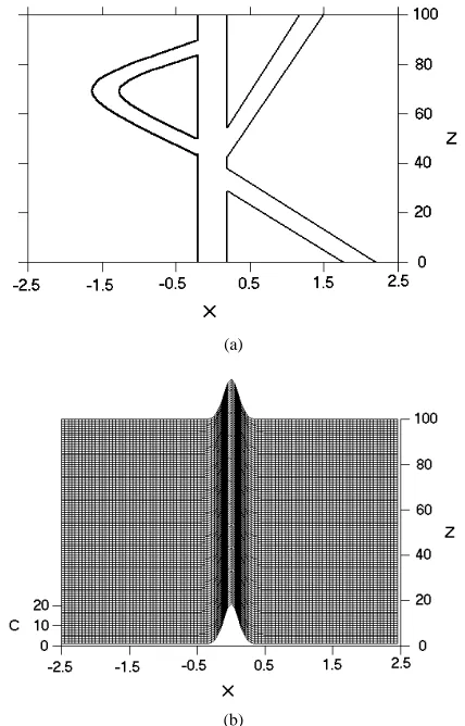
The geometry of the designed structure is shown in Figure 6(a).
Let us analyse the results of the numerical simulations for the three possible input combinations to demonstrate the correctness of the developed theory, neglecting the situation of no inputs that represents the first combina-tion according to Table 1.
In Figure 6(b) the numerical simulation in case of the presence of the only input pulse at the entrance 1 (the second input combination of Table 1) is shown. In this case, since the refractive index variation is equal to the one of the delay branch, the beam propagates undis-turbed and reaches the output, generating a proper phase coded pulse.
In Figure 6(c) the numerical simulation of the third input combination, that is the presence of only an input pulse at the entrance 2 is shown. In this case, the pulse first propagates properly trapped inside the secondary waveguide, due to the fact that the parameters of the structures have been designed to lock it. It reaches the main waveguide, with a certain phase difference that we
have designed to be equal to 0.55 , reaching the output, and generating a proper output phase coded pulse.
In Figure 6(d) the numerical simulation of the fourth input combination, that is the presence of both input pulses at the entrances is shown. In this case, the two pulses meet at the merging point between the main waveguide and the secondary waveguide with a relative phase difference greater than 0.55 , that is in a repulsive situation. The two beams propagate parallel each other properly separated, until reaching the bifurcation point. In this zone the pulse relative to input 1 is pushed into the delay branch, while the pulse relative to input two is pushed inside the drain waveguide where it reaches the drain output. The first pulse, that propagates inside the delay branch, is trapped inside it since the structure has been properly designed and enters again inside the main waveguide with a relative designed phase difference equal to 1.24 , reaching the output and generating a proper output phase coded pulse.
The numerical simulations, as shown in Figures 6, confirm the theory developed.
5. A Numerical Design of the Device
We want now to give a numerical example for the design
(a)
[image:7.595.316.530.386.720.2]242 F. GARZIA ET AL.
(c)
(d)
Figures 6. Upper view and numerical simulations. The pa-rameters of the waveguide are a=16.9, d=1.4, b=0.25,
Δn=1·10-5. (a) Upper view of the structure; (b) Numerical simulation of the behaviour of the structure in the presence of the only input 1; (c) Numerical simulation of the behav-iour of the structure in the presence of the only input 2; (d) Numerical simulation of the behaviour of the structure in the presence of both input 1 and input 2.
of the considered device.
Suppose we have a Schott B 270 glass, whose optical parameters at 0620nm
/W n
are 0 and
being 0 and 2 are the linear
and nonlinear refractive indices respectively [17]. Let us consider a spot size of the beam equal to
1.53
n
10
d
20 2
2 3.4 10 m
n n
0 m.
The design rules are very restrictive in a real situation since it is necessary to match different requests with a reduced free choice of parameters. In fact once fixed the source and the proper material for the given source it is necessary to design the geometry of the structure to trap the pulses with a proper soliton intensity level, generat-ing the necessary coded phase variation. Further, since we use the same constructive technology, we suppose
that the refractive index variation 0 is the same for
the delay branch and for the secondary waveguide, in-troducing another restriction.
n
It is well known that, given a certain material and a certain light source, the intensity necessary to generate a soliton beam is given by:
0
2 2
0 2
2
s n I
d n
(25)
where is the wavevector of the beam. Substituting the numerical values into (25) we have
15 2
3.74 10 /
s
I W m .
Since the intensity of the beam Is is related to its
amplitude C from [12-14]:
2 0 2 21
2
log 2 3
s
n
I C
n
(26)
it is possible to express (11) and (23) in term of the in-tensity of the beams.
We choose for example and we start with the design of the device.
2 0 1 10
n
We want to code the third situation (only a pulse at the input 2) with a relative phase variation just greater than
/2 and the fourth situation (both the input pulses) with a relative phase very close to .
We choose d 2d020m
.96 m
. Substituting this value into Equation (15) we obtain a=0.0639. In this way the geometry of the delay branch is totally defined. If we choose b19 , using (11) and (26) we obtain a lock-in value 1.25 1016
D
2 /
I W m , that is a value above the soliton threshold calculated with (25) and be-low the second order soliton threshold.
We have now to check if, with these values, we have obtained a phase difference value very close to , as we desire. The phase difference value can be calculated as the product of the wavevector and the difference of path between the delay branch and the main waveguide. Us-ing (20), we obtain 0.59 . This value is very close to the other phase value, generating two phase val-ues very close each other. In this case it is necessary to make some correction to the geometry of the delay branch to correct the phase value to a value close to , keeping at the same time the lock-intensity above the soliton generation threshold. We choose to increase the value of the "a" parameter, that allows the paraxial ap-proximation to be conserved. If we increase this parame-ter by 1.53 times, the total length of the delay branch increases. The new intensity lock-in value decreases to
15 2
5.36 10 /
D
243
It is now necessary to project the secondary input waveguide. We want to obtain the same intensity lock-in value calculated for the delay branch and a phase differ-ence value a bit greater than /2.
This kind of waveguide as already been studied [13] showing a behaviour similar to the parabolic waveguide and a lock-in value equal to:
1 2 0v
2
G D C
n
(27)
where is the tangent of the inclination angle with respect to the longitudinal direction. It is obviously nec-essary to respect, even in this case, the paraxial approxi-mation; this means that once we have chosen the distance
vG
L
a between the second input and the main input, the longitudinal length bL of the waveguide cannot be
shorter than a minimum, calculated according to the paraxial limit, that is:
tan 8 0.14
L L
a b bL (28) Since we suppose to generate this waveguide using the same physical procedure used for the delay branch, we have to suppose that the value is the same for both the waveguides. If we use as a first attempt value L , to generate a device whose lateral
exten-sions with respect to the main waveguide are the same, we immedi tely obtain
2 0 1 10
n
a d
a bL from (28), that allows us to
calculate . Substituting these values into (27), using (26) we have an intensity lock-in value equal to
G
v
2.23 1017 / 2
DS
I W m and S 1.12
d
. The wave- guide designed according to these criteria is totally use-less for our purpose since the lock-in value is greatly above the generation value of a second order soliton and consequently above the lock-in value calculated for the delay branch. Further, the phase value obtained is totally different with respect to the one we desire. It is therefore necessary to find another approach. If we impose the waveguide to have the same lock-in intensity of the delay branch, considering always aL , we can calculate
L b
5650
b
, reversing the reasoning followed above. In this case we obtain L m that satisfies the paraxial
con-dition expressed by (27). If we calculate the phase dif-ference we have S 0.175, that is not only a
dif-ferent value with respect to the desired one but also a value that does not allow the repulsion between the two beams, that is a fundamental condition to make the de-vice operate correctly.
Consequently it is necessary to act also on aL,
con-sidering a device that has not the same lateral extension with respect to the main waveguide. Fixing the intensity lock-in level to be equal to the one of the delay branch and fixing the phase difference S to be as close as
possible to 0.5 , it is possible to demonstrate that a valid
waveguide is the one characterised by aL 3d 60m
and bL 16935m, that provides a phase difference
S 0.53
, respecting the paraxial condition ex-pressed by (27).
The problems found in the design of the secondary input waveguide could be avoided if we could act also on
0 n
, but this is very difficult to be made in a real situa-tion where both the delay branch and the inclined waveguide are generated in the same process.
Different approaches can be used to design the device, as for example, to dimension first the secondary wave- guide and the delay branch, but they are always sub-jected to different restrictions due to the physics of the waveguides generation process.
6. Temporal Considerations
Further considerations about the temporal behaviour and the absorbing behaviour of solitons in transverse refrac-tive index profile device have already been studied [13,14] and they are not repeated here for brevity.
Since the response time of the considered material are of the order of femtoseconds, the proposed device can reach operative velocity of the order of thousands of Gbit/s and it is limited only by the operative velocities of the actual sources.
7. Conclusions
We have studied and designed an all-optical crypto-graphic device, whose working principles are based on the repulsive and propagation properties of solitons in a parabolic transverse refractive index profile, that we deeply analysed in the paper.
The switching properties have been studied in details, obtaining some useful design criteria for a practical de-vice.
The device can be properly designed by means of the geometrical and optical parameters of the different structures that compose the modulator.
Due to its peculiar features, the only limit to its maxi-mum operative velocity is represented by the maximaxi-mum repetition rate of the input sources.
8. References
[1] R. Y. Ciao, E. Garmire and C. H. Townes, “Self-Trapping of Optical Beams,” Physical Review Letters, Vol. 13, No. 15, 1964, pp. 479-482.
244 F. GARZIA ET AL.
[3] W. Krolikowski and Y. S. Kivshar, “Soliton-Based Optical Switching In Waveguide Arrays,” Journal of the Optical Society of America B, Vol. 13, No. 5, 1996, pp. 876-887.
[4] N. N. Akhmediev and A. Ankiewicz, “Spatial Soliton X-Junctions and Couplers,” Optics Communications, Vol. 100, No. 1-4, 1993, pp. 186-192.
[5] W. Krolikowski, X. Yang, B. Luther-Davies and J. Breslin, “Dark Soliton Steering in a Saturable Nonlinear Medium,” Optics Communications, Vol. 105, No. 3-4, 1994, pp. 219-225.
[6] A. P. Sheppard, “Devices Written by Colliding Spatial Solitons: A Coupled Mode Theory Approach,” Optics Communications, Vol. 102, No. 3-4, 1993, pp. 317-323.
[7] J. P. Gordon, “Interaction Forces among Solitons in Optical Fibers,” Optics Letters, Vol. 8, No. 11, 1983, pp. 596-598.
[8] F. Garzia, C. Sibilia, M. Bertolotti, R. Horak and J. Bajer, “Phase Properties of a Two-Soliton System in a Non Linear Planar Waveguide,” Optics Communications, Vol. 108, No. 1-3, 1994, pp. 47- 54.
[9] A. B. Aceves, J. V. Moloney and A. C. Newell, “Reflection and Transmission of Self-Focused Channels at Nonlinear Dielectric Interfaces,” Optics Letters, Vol. 13, No. 11, 1988, pp. 1002-1004.
[10] P. Varatharajah, A. B. Aceves and J. V. Moloney, “All-Optical Spatial Scanner,” Applied Physics Letters,Vol. 54, 1989, pp. 2631-2633.
[11] A .B. Aceves, et al., “Particle Aspects of Collimated Light Channel Propagation at Nonlinear Interfaces and in Waveguides,” Journal of the Optical Society of America B, Vol. 7, No. 6, 1990, pp. 963-974.
[12] F. Garzia, C. Sibilia and M. Bertolotti, “Swing Effect of Spatial Soliton,” Optics Communications, Vol. 139, No. 4-6, 1997, pp. 193-198.
[13] F. Garzia, C. Sibilia and M. Bertolotti, “High Pass Soliton Filter,” Optics Communications, Vol. 152, No. 1-3, 1998, pp. 153-160.
[14] F. Garzia, C. Sibilia, and M. Bertolotti, “All optical soliton based router”, Opt. Comm., vol. 168/1-4, pp. 277-285, 1999.
[15] H. W. Chen and T. Liu, “Nonlinear Wave and Soliton Propagation in Media with Arbitrary Inhomogeneities,” Physics of Fluids, Vol. 21, No. 3, 1978, pp. 377-380.
[16] P. K. Cow, N. L. Tsintsadze and D. D. Tsakhaya, “Emission of Ion-Sound Waves by a Langmuir Soliton Moving with Acceleration,” Soviet Physics-JETP, Vol. 55, 1982, pp. 839- 843.
[17] J. S. Aitchison, et al., “Observation of Spatial Optical Solitons in a Nonlinear Glass Waveguide,” Optics Letters, Vol. 15, No. 9, 1990, pp. 471-473.
[18] P. Refreiger and B. Javidi, “Optical Image Encryption on Input Plane and Fourier Plane Random Encoding,” Optics Letters, Vol. 20, No. 7, 1995, pp.767-769.
[19] O. Matoba and B. Javidi, “Encrypted Optical Memory System Using Three-Dimensional Key in the Fresnel Domain,” Optics Letters, Vol. 24, No. 11, 1999, pp.762-764.
[20] J. W. Han, C. S. Park, D. H. Ryu and E. S. Kin, “Optical Image Encryption Based on XOR Operations,” Optical Engineering (Bellingham), Vol. 38, No. 1, 1999, pp. 47-54.
[21] J. W. Han, S. H. Lee and E. S. Kin, “Optical Key Bit Stream Generator,” Optical Engineering (Bellingham), Vol. 38, No. 1, 1999, pp. 33-38. [22] S. T. Liu, Q. L. Mi and B. H. Zhu, “Optical Image
Encryption with Multistage and Multichannel Fractional Fourier-Domain Filtering,” Optics Letters, Vol. 26, No. 16, 2001, pp. 1242-1244.
[23] Y. Zhang, C. H. Zheng and N. Tanno, “Optical Encryption Based on Iterative Fractional Fourier Transform,” Optics Communications, Vol. 202, No. 4-6, 2002, pp. 277-285.
[24] A. Carciner, M. Montes-Usategui, S. Arcos and I. Juvells, “Vulnerability to Chosen-Cyphertext Attacks of Optical Encryption Schemes Based on Double Random Phase Keys,” Optics Letters, Vol. 30, No. 13, 2005, pp. 1644-1646.
[25] U. Gopinathan, D. S. Monaghan, T. J. Naughton and J. T. Sheridan, “A Known-Plaintext Heuristic Attack on the Fourier Plane Encryption Algorithm,” Optics Express, Vol. 14, No. 8, 2006, pp. 3181-3186.
[26] Y. Frauel, A. Castro, T. J. Naughton and B. Javidi, “Resistance of the Double Phase Encryption against Various Attacks,” Optics Express, Vol. 15, No. 16, 2007, pp. 10253-10265.
[27] P. K. Wang, L. A. Watson and C. Chatwin, “Random Phase Encoding for Optical Security,” Optical Engineering (Bellingham), Vol. 35, No. 9, 1996, pp. 2464-2469.
[28] Y. Li, K. Kreske and J. Rosen, “Security and Encryption Optical Systems Based on a Correlator with Significant Output Images,” Applied Optics, Vol. 39, No. 29, 2000, pp. 5925-5301.
[29] Z. J. Liu and S. T. Liu, “Double Image Encryption Based on Iterative Fractional Fourier Transform,” Optics Communications, Vol. 275, No. 2, 2007, pp. 324-329.
[30] B. Javidi and T. Nomura, “Securing Information by Use of Digital Olography,” Optics Letters, Vol. 25, No. 1, 2000, pp. 28-30.
245
[32] X. F. Meng, X. Peng, L. Z. Cai, A. M. Li, Z. Gao and Y. R. Wang, “Cryptosystem Based on Two Step Phase-Shifting Interferometry and the RSA Pubblic-Key Encryption Algorithm,” Journal of Optics A: Pure Applied Optics, Vol. 11, No. 8, 2009, pp. 85402-85410.