doi:10.4236/epe.2011.31003 Published Online February 2011 (http://www.SciRP.org/journal/epe)
Cost Control of the Transmission Congestion Management
in Electricity Systems Based on Ant Colony Algorithm
Bin Liu, Jixin Kang, Nan Jiang, Yuanwei Jing
Faculty of Information Science and Engineering, Northeastern University, Shenyang, China E-mail: jiangnan@ise.neu.edu.cn
Received October 8, 2010; revised November 3, 2010; accepted November 4, 2010
Abstract
This paper investigates the cost control problem of congestion management model in the real-time power systems. An improved optimal congestion cost model is built by introducing the congestion factor in dealing with the cases: opening the generator side and load side simultaneously. The problem of real-time congestion management is transformed to a nonlinear programming problem. While the transmission congestion is maximum, the adjustment cost is minimum based on the ant colony algorithm, and the global optimal solu-tion is obtained. Simulasolu-tion results show that the improved optimal model can obviously reduce the adjust-ment cost and the designed algorithm is safe and easy to impleadjust-ment.
Keywords: Electricity Systems, Congestion Management, Ant Colony Algorithm, Minimax, Adjustment Cost
1. Introduction
With the open of transmission network, the problem of transmission congestion becomes very serious under power market environment. When the active tidal current in line surpasses the limiting value, the net side will adjust various units’ output allocative decision to avoid transmission con- gestion as much as possible for safety [1-3]. When the unit output distribution plan is adjusted, the transaction cost of network side will rise due to the emergence of congestion cost. However, adjustment schemes in many cases are not unique, different adjustment programs will lead to different congestion costs, so there exists an optimal strategy [4-7]. It is important that how to choose the optimal adjustment program to ensure the loss caused by network’s plan failure is the least [8,9].
Reference [4,10,11] studied congestion management al-gorithm problem and power system economic dispatch problem, but the optimization models considered do not cover the cost of load side. Reference [12] designed a rela-tively simple regulation for blocking costs against the op-timization model of transmission congestion management. Reference [13,14] proposed a kind of generator adjustment expense smallest optimization model. Reference [15] pro-posed an optimization model using sensitivity factor to solve the blocking problem existing regional electricity market based on AC power flow model.
However, these traditional optimizations of transmission congestion mostly focused on the trend of the objective function or as a percentage of the basic constraints to the introduction of the congestion management model. This approach increases the difficult to solving the model in virtually.
This paper presents the congestion cost optimal models for the case: open the generate side and the load side at the same time. The greatest feature of this model is that the power flow percentage is involved in the calculation of blocking cost in order to make the power flow limit’s li-ability more clearly. The optimal solution is obtained by using the ant colony algorithm which has the global search ability. Finally, the model is simulated for two cases: the load of 982.4 MW and 1052.8 MW. Simulation results show that the improved optimal model can obviously re-duce the cost of electricity.
2. Problem Statement
Congestion management is a complicated systematic work, including the interest of the generate side and the load side at the same time.
Transmission congestion management principles: 1) Transmission congestion is eliminated by adjusting the unit output distribution program.
B. LIU ET AL. 18
the safety margin transmission in line to avoid power cuts (focus to reduce the load demand) , but make sure that the percentage of the absolute value of the trend ex-ceeding the limit value in each line is as small as possi-ble.
3) If the percentage of the absolute value of the trend exceeding the limit value in each line is greater than rela-tive safety margin no matter how to distribute the unit output, the power should be cut in the load side.
3. Congestion Management Optimal Model
Traditional congestion management model based on nodal price has a strong practical, but the model con-straints have nonlinear expressions, which makes solving the biggest problem. Because the trends affect the cost of congestion management based on the generator side, the traditional model needs quadratic programming, which means complex. When there is interruptible load in the load side, the model only focuses on the minimum power purchase cost of the network and more importantly it doesn’t reflect the current contribution of the obstruction charges. Therefore, this paper will improve the inter-ruptible load with opening the generator side and load side simultaneously, focusing on the influence to conges-tion cost when the trend is inevitable. The new model’s objective function is the minimum congestion cost.
3.1. Current Ratio Factor
Generally, researchers use the percent of effective power flow exceeding the safe threshold value in each line to measure the congestion degree, here called transmission congestion rate. It could be expressed as:
k k k
k
y u
u
(1)
where k represents the effective power flow in the
main lines in power network, k represents the limited
value of power flow in the wiring, which means security margin in the wiring, .
y
u
,
k1, s
Obviously, when the effective power flow is smaller than the safe threshold value, then k 0; when the effective power flow exceeds the safe threshold value, then k 0. Let maxk, k1,,s. We study the
state when the transmission congestion is maximum. Therefore is a positive number in this paper.
The power flow describes the distributions of voltage (including the amplitude and phase), active power and reactive power in power network. Assume there are eight generators and six main lines. It can be seen from the observation data that active power flow
1, 2, ,k
y k
1, 2, , is
and the generator outputx i n
i
are linear relation- ship as follows,
1
n i
k k
i
y x
(2)
where i k
represents the linear relevant coefficient of the active power flow relating to the output of each gen-erator.
3.2. The Improved Transmission Congestion Control Model
The influence of power flow on congestion cost can’t be reflected fully when only power flow violation is taken as the constrain condition. Therefore, transmission con-gestion rate (power flow proportion coefficient) is intro-duced into the target function of cost model in this paper. The congestion cost is larger with the increase of the proportion coefficient. The responsibility of the power flow violation can be ascertained by using the assump-tion, and the partners of power market can be constrained and the process of solution can be simplified. It has the direct meaning to the commercialization of power market.
The goal of real-time congestion management is to eliminate the congestion with the minimum cost. In this section, we consider the two cases: generation bidding only, and generation and auxiliary power bidding at the same time. Considering the adjustment of the minimum cost as the target function, the optimal model can be in-vestigated when the transmission congestion rate is as large as possible.
If the transmission congestion rate is beyond the safe margin, the worst congestion occurs. Then we should adjust the output plan and interrupt parts of the load and compensate for it. The congestion cost including the compensation fee paid for consumers. In order to get the minimum of the sum of adjustment cost, the generator and load side should be adjusted simultaneously.
Assumption Qj is the compensation price for the
reason of power interruption, j is the adjusted
inter-ruption load, and then jQj is the compensation fee for
the reason of power interruption. Considering the effect of power flow coefficient on congestion cost, the target function can be defined as follows:
*
1,2, , 1 1
min max k n i i l j j
i n i j
J P Q
(3)
1 1 1 0 . . i n i i n i i
i i i i s
i ij ij j
x B
s t
C TV x C TV
x x d
gen-erator in the distribution preplan, i represents the
corresponding price of i
i P
x which locates the generator s the adjusted distribution replant,
i is the change
value of generator of adjusted output plan com-pared with original plan after the congestion happen. is the number of the consumers who participate the in-terruption load management and bid successfully in
i
l
ancillary service market. is the total amount of gen-erators that participate in the output adjustment.
n
s is the number of main lines, is the load requirement of next time-interval forecast, i s the output of generator
, i s the length of one time-interval, i is the climb
rate, ij is the interval capability from generator to
generator .
B C i T d V i j xij is defined as follows:
1 output of - ne h rval
0 out output o -th g e-inter
ij
x
th ge f rato ene r in rator
i j-t
in tim -t i j e-inte h tim with val
where i2,, ,n j1,2,,s. Constraint conditions 1 n i i x B
and1 n i i
0C TV
ensure the load forecasting always to meet the require-ments, i.e. the adjustment of each generator output al-ways to meet the load requirements when the require-ment is . Constraint condition i i i i
describes the generator climb rate i.e. if the output is i
at present, in the next time-interval the generator set output will lies within the range of
B TVi
C
x C
,i i i
C TV C TVi .
Constraint condition
1
s i ij ij
j
x x d
restricts the capability of generator output, i.e. the gen-erator output can’t exceed the sum of every time-interval output.
Remark 1: the vector will increase correspondingly with the increase of the rate of transmission congestion. As a result, the adjustment cost will increase. However, our final goal is to reduce the congestion cost. Then this problem could be considered as a typical mini-max problem. We will solve the set models in the following section to verify their security and reliability.
4. Model Solution
4.1. Characteristics of Ant Colony Algorithm
1) Positive feedback mechanism. The more ants after the path chosen by the ants follow-up more likely, by con-tinuously updated information on the optimal path of Convergence.
2) Generality. The algorithm model has a good adapta-tion for other optimizaadapta-tion problem.
3) Distributed parallel computing. The algorithm sear- ches solution in the global context of multi-location si-multaneously. It is a global optimization heuristic algo-rithm, both for single objective optimization problem and
for multi-objective optimization or constrained optimiza-tion problem condioptimiza-tions.
4.2. Transmission Congestion Model Based on Improved Ant Colony Algorithm
Based on the improved congestion management model, the model’s objective function value is set to the shortest path on which ants find food. Above the analysis, we can reach a conclusion: ant colony algo-rithm solving process has the two major cycles. Circu-lation is controlled by the change of cities’ number while the outer loop is controlled by the change of ants’ number. The parameters have a significant impact on path of ants searching food.
1) Initial control parameter is chosen as large as possi-ble.
2) Attenuation function controls the ants’ number. It is defined as follows: M kd*M. Where d is close to 1. This value is closer to 1 that participate in the more ants find food, the better the optimal solution obtained, because it determines the number of outer loop.
k
3) There are many options to terminate the conditions. A variety of conditions on the performance of the algo-rithm has great influence on the quality of reconciliation. This paper sets the number of iterations and comparison as both internal and external conditions.
The ant colony algorithm process of the improved blocking model:
1) Initialization of variable. Set M ants, cities (units) and pheromone matrix system be 1. In this paper, we suppose there are eight generating units and six transmission lines.
N
M
2) Set ants to cities. Generate an initial solu-tion set (the starting point for the algorithm) according to the constraints random variable of the improved model (the output of new programs).
N
1, 2, , n
X x x x is the output matrix of redistribution preplan of generators. Firstly, restrict the output of generator n within the range of
n, n
according to the known data and ine-quality constraint conditions. Where,
a b
, n
B. LIU ET AL. 20
section of
CnTVn, Cn TVn
and 1s n nj
j nj
x x d
. Antcolony.
3) Algorithm has a major advantage which is the final result of optimization has nothing to do with the initial value. So with the generated solution
is set with the random number. It shows as follows: . At the same time, we can use the other output to express the output of genera-tor in order to satisfy the equation constraint condi-tion:
1, 2, , 7 ix i
0,1
i i i i
x a b a random
n
8 1 2 3 4 5 6 7
x B x x x x x x x
4) M ants select to the next city with a certain
probability to complete their tour, so the new output scheme is obtained. The congestion cost of the new and the corresponding output program’s difference is called evaluation function: * *
11 1
J J J
.
5) If the evaluation function is a negative number, the current efforts contributing to the program is accepted to the new program; else, accept it as the new one accord-ing the probability:
1
0,1
k i
p k
p random
p k
The new program is the local optimal solution. Where
ij ijp k L
is a sequence consisting of after some iterative optimizations.
p k
6) The number of the searching city increasing, from
to , pheromone is updated.
Deter-mine whether the conditions meet the above. Jump out of circulation and turn to the next step when it doesn’t meet. Repeat the two steps above until the maximum number of iterations and record the best path in this iteration.
j j j
1, 2,,n
7) The number of foraging ants increasing, record every round each ant foraging route and feeding distance, which means the unit costs under the current combined output. Select the minimum number of optimal solutions and repeat (3-6) steps until reaching the maximum num-ber of iterations.
8) Getting results. By the Step 3 and Step 4, get the optimal distance of each ant, step 3 and 6 control the change of the size of M , to seek the global optimal so-lution.
5. Simulation Examples
According to the characteristics of Ant Colony
Algo-rithm, the three examples will be simulated, combining with the proposed model. Main purpose is to compare the costs resulting from the current output matrix with costs resulting from the previous output matrix, and choose the smaller the cost. Finally, Minimum cost is found and after a finite number of iterations, and it as an optimal solution of the example.
5.1. Example 1: Load Requirement is 982.4 MW
[image:4.595.309.536.552.618.2]We identify the simple feasibility and safe reliability of the proposed congestion optimal model by simulation examples.
Table 1 gives the output of each generator and the cor-responding climb rate. Table 2 gives the output distribu-tion preplan and corresponding price each generator when the load forecasting is 982.4 MW.
If the output preplan does not change, i.e., the output of each generator according to Table 1, this preplan is decided by the transaction rules of power market.
Let maxk 0.22 According to the safety and trans-action rules of power market, we can get the original cost “¥597.694” for the increase of load requirement by the formula.
Then we resolve the preplan aiming to minimize the preplan cost using the simulation annealing algorithm. Where, let the current output matrix
120, 73,180,80,125,125,81, 90
c , the revolution of the
generator unit v
2.1,1, 3.1,1.3,1.8,2,1.4,1.8
, the target output f
150, 79,180, 99.5,125,140, 95,113.9
, the price
252, 300, 233, 302, 215, 252, 260
.95
, 303 , the
p
phero-mone parameter 0 .
The simulation result is as follows:
The X-axis represents the iteration times and the Y-axis represents the target function.
It can be seen from Figure 1 that the cost is
¥478.5872 and the saving cost is ¥119.106. The out-
Table 1. The present climb rate of each generator output.
1 2 3 4 5 6 7 8
Present
output (MW) 120 73 180 80 125 125 81.1 90
Rate
[image:4.595.309.537.655.721.2]MW/min 2.1 1 3.1 1.3 1.8 2 1.4 1.8
Table 2. The distribution preplan each generator when load forecasting is 982.4 MW.
1 2 3 4 5 6 7 8
Forecasting
outpout MW 150 79 180 99.5 125 140 95 113.9
Price
Figure 1. The adjustment cost when load is 982.4 MW.
put of each generator is as follows:
147.3545, 69.1272, 228.5268, 64.0073,
149.2004,155.6027,101.9507, 66.6304
X
We can see that the process of decreasing temperature is reasonable and the annealing can jump out the local optimal solution. Therefore, the final minimum value is reliability after enough iteration times.
5.2. Example 2: Load Requirement is 1052.8 MW
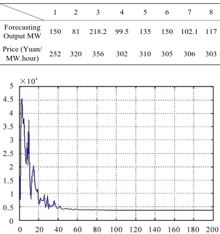
Table 3 gives the output distribution preplan when the load requirement is 1052.8 MW. Let maxk 0.22. According to the safety and transaction rules of power market, we can get the original cost “¥3845.814” for the increase of load requirement. Where, let the current out-put matrix c
150,81, 218.2, 99.5,135,150,102.1,117
, the revolution of the generator unit
2.1,1, 3.
v
150, 791,1.3,1.8, 2,1.4,1.8 , the target output
f
252, 30,180, 99.5,125,140, 95,113.9
, the price p 0, 233, 302, 215, 252, 260, 3030.95
, the pheromo- ne parameter .
The simulation result using matlab is as follows: The X-axis represents the iteration times and the Y-axis represents the target function.
It can be seen from Figure 2 that the cost is ¥3784.6 and the saving cost is ¥61.214. The output of each generator is as follows:
151.9448,83.9114,197.8033, 97.7498,
151.4479,156.3922,102.4476,118.8128
X
[image:5.595.63.281.77.238.2]We can also see form Figure 2 that the larger load re-quirement corresponds the higher generator cost. There-fore, we consider the method of interruptible load in or-der to realize the cost management of high load require-ment.
Table 3. The generator forecasting output when load re-quirement is 1052.8 MW.
1 2 3 4 5 6 7 8
Forecasting
Output MW 150 81 218.2 99.5 135 150 102.1 117
Price (Yuan/
[image:5.595.310.536.102.343.2]MW.hour) 252 320 356 302 310 305 306 303
Figure 2. The adjustment cost when load is 1052.8 MW.
5.3. Example 3: Simulation of Interruptible Load Model
Assume the present output is described by Table 1, the load requirement is 1052.8 MW. The consumer side ex-ists the interruptible load according to the interrupt agreement, and the interruptible quantity is 30.4 MW. Because of the implementation of interruptible load, the distribution preplan of each generator output can be en-forced according to the residual load requirement. At the same time, corresponding maxk 0.02, load require-ment decrease dramatically compare with the 1052.8 MW. Where, let the current output matrix
120, 73,180,80,125,12
c 5,81, 90 , the revolution of the
generator unit v
2.1,1,3.1,1.3,1.8, 2,1.4,1.8
, the target output f
150, 79,180,99.5,125,140, 95,113.9
the price,
252, 300, 233,
p 302, 215, 252, 260
0.95
, 303 , the pheromone parameter .
The compensation fee for the interrupt is calculated as follows:
1 max
0.02 25.86 4000 3.5 541 1.04 154
2109.8732
l k j j
j
Q
The simulation result using MATLAB is:
B. LIU ET AL. 22
Figure 3.The adjustment cost when consumer side exist the interruptible load.
We can get the result using the calculation function of MATLAB, the generator cost is ¥2592.701. The gen-erator cost decreases dramatically compare with
¥3780.9 without the interruptible road. The saving cost is ¥1188.199.The output of each generator is as fol-lows:
153.1424, 65.5055, 227.4673, 61.3641,
151.0063,145.5638,101.3008, 79.0498
X
Therefore, signing the appropriate interruptible load agreement can decrease the congestion cost and improve the social benefits.
6. Conclusion
In this paper, an improved optimal congestion cost model is built by introducing the congestion factor in dealing with the cases: opening the generator side and load side simultaneously. The optimal solution is obtained based on the ant colony algorithm. The model is simulated for two cases: the load of 982.4 MW and 1052.8 MW. The results show that the model can significantly reduce the cost of electricity. As the load demand increasing, a cor-responding increase in congestion costs, the effective interruptible load is used to reduce the cost and control the adjustment effectively.
7. Acknowledgment
This work is supported by the Fundamental Research Funds for the Central Universities, under grant 090304004, and the National Natural Science Foundation of China, under grant 60274009, and Specialized Re-search Fund for the Doctoral Program of Higher
Educa-tion, under grant 20020145007.
8. References
[1] Y. S. Wei, X. N. Wang and T. M. Li, “Power Transmis-sion Management Modeling in the Electricity Power Mar-ket,” Zhejiang Electric Power, Vol. 26, No. 4, 2005, pp. 14-16.
[2] R. D. Christle and B. F. Wollenberg, “Wangensteen. Transmission Management in the Deregulated Environ-ment,” IEEE Transactions on Power System, Vol. 15, No. 2, 2000, pp.171-195.
[3] H. Singh, S. Hao and A. D. Papalexopoulos, “Transmis-sion Congestion Management in Competitive Electricity Markets,” IEEE Transactions on Power Systems, Vol. 13, No. 2, 1998, pp. 672-680.
[4] Z. Q. Wu, M. M. Zhu and L.Y. Wang, “Online Transmis-sion Congestion Management Model and Algorithm,” Proceedings of the Chinese Society of Universities for Electric Power System and Automation, Vol. 19, No. 6, 2007, pp. 109-113.
[5] J. S. Hu, L. M. Zhou and S. L. Sui, “Transmission Con-gestion Management of Electricity Markets and Programs of Matlab,” Journal of Qingdao Technological University, Vol. 28, No. 1, 2007, pp. 91-95.
[6] W. M. Mao, M. Zhou and G. Y. Li, “Multi-Period Power Transmission Congestion Management Considering In-terruptible Loads,” Power System Technology, Vol. 32, No. 4, 2008, pp. 72-77.
[7] Y. P. Zhang, L. W. Jiao and S. S. Chen, “A Survey of Transmission Congestion Management in Electricity Mar- kets,” Power System Technology, Vol. 27, No. 8, 2003, pp. 1-9.
[8] G. B. Shrestha and P. A. J. Fonseka, “Congestion-Driven Transmission Espansion in Competitive Power Markets,” IEEE Transaction on Power System, Vol. 19, No. 3, 2004, pp. 1658-1665. doi:10.1109/TPWRS.2004.831701
[9] R. Mendez and H. Rudnick, “Congestion Management and Transmission Rights in Centralized Electric Mar-kets,” IEEE Transaction on Power System, Vol. 19, No. 2, 2004, pp. 889-896. doi:10.1109/TPWRS.2003.821617
[10] M. M. Zhu, Z. Q. Wu and S. S. Ye, et al, “Transmission Congestion Management Model and Algorithm Based on Generating Unit Power up and down,” Modern Electric Power, Vol. 24, No. 1, 2007, pp. 68-71.
[11] Z. L. Yi, “The Optimize Model on Management of Trans- mit Electricity Block in the Electric Power Market,” Journal of Hengyang Normal University, Vol. 27, No. 3, 2006, pp. 22-25.
[12] J. Lei, Y. Deng and R. Zhang, “Congestion Management for Generation Scheduling in a Deregulated Chinese Po- wer System,” IEEE of Power Engineering Society Winter Meeting, 2001, pp. 1262-1265.
2002, pp. 10-13.
[14] A. Kumar, S. C. Sristava and S. N. Singh, “A Zonal Con-gestion Management Approach Using AC Transmission Congestion Distribute Factor,” Electric Power Systems Research, Vol. 72, No. 1, 2004, pp. 85-93. doi:10.1016/
j.epsr.2004. 03.011