ISSN Online: 2164-5175 ISSN Print: 2164-5167
DOI: 10.4236/ajibm.2019.94065 Apr. 26, 2019 950 American Journal of Industrial and Business Management
Efficiency Analysis of Electricity, Thermal
Power Production and Supply Industries in
China
Xuefeng Jiang
Department of Economics, Jinan University, Guangzhou, China
Abstract
In this paper, the input-oriented distance function is applied to the efficiency analysis of China’s electricity, thermal power production and supply indus-tries. Due to the obvious gap between China’s east, central and west, we use the metafrontier method to divide the data into three parts according to east, central and west. On the basis of the previous research, this paper makes some innovations in the estimation method, that is, using the two-stage linear programming method to estimate the common boundary input distance function. The results show that the technical efficiency of the eastern, central and western regions is significantly different, which is mainly reflected in that the technical efficiency of the eastern region is higher than that of the central and western regions, and the efficiency gap between the three regions shows no signs of narrowing during the “eleventh five-year plan” and “twelfth five-year plan”. Therefore, the electricity, thermal power production and supply industries in central and western China still need to change the devel-opment mode and improve the develdevel-opment quality.
Keywords
Input Distance Function, Metafrontier, Efficiency, Two-Stage Linear Programming
1. Introduction
Electricity, thermal power production and supply industry is the basic pillar in-dustry for national economic development. Specifically, the inin-dustry that we will study includes the electricity industry and thermal production and supply in-dustry. Electric power is the power of modern economic development. It pro-vides energy supply and power support for the development of various indus-How to cite this paper: Jiang, X.F. (2019)
Efficiency Analysis of Electricity, Thermal Power Production and Supply Industries in China. American Journal of Industrial and Business Management, 9, 950-973.
https://doi.org/10.4236/ajibm.2019.94065
Received: April 3, 2019 Accepted: April 23, 2019 Published: April 26, 2019
Copyright © 2019 by author(s) and Scientific Research Publishing Inc. This work is licensed under the Creative Commons Attribution International License (CC BY 4.0).
http://creativecommons.org/licenses/by/4.0/
DOI: 10.4236/ajibm.2019.94065 951 American Journal of Industrial and Business Management tries in the national economy. Industrial production and people’s daily life are inseparable from electric power. The power industry maintains a high correla-tion with the macro-economy, and the growth rate of power produccorrela-tion and power consumption changes with the change of GDP growth rate. Industrial production and people’s daily life cannot be separated from the electric energy and heat energy provided by the industry. According to China Statistical Year-book, from 2001 to 2013, driven by the rapid development of national economy and the electricity demand brought by industrialization and urbanization, the national electricity demand maintained an average annual rate of 11.22%. The thermal power production and supply industry refers to the activities of using coal, oil, gas and other energy resources to produce steam and hot water through boilers and other devices, or outsourcing steam and hot water for supply and sales, maintenance and management of heating facilities. It is a key industry supported by the state in the field of capital construction. The thermal produc-tion and supply industry is extremely important for areas needing heating in winter, and is also deeply associated with basic industries such as power, con-struction and coal. China’s “twelfth five-year” plan which is an important eco-nomic development plan involves the industry’s development and reform, such as “energy twelfth five-year planning” indicating the developing direction of the thermal power cogeneration, “building energy saving special planning during twelfth five-year” put forward to deepen the reform of the heating system, im-plementation of heating metering, promoting energy-saving renovation of existing buildings in northern heating metering and energy-saving ability of 27 million tons of standard coal, the “plan for heat metering heating in the north area for existing residential buildings during twelfth five-year” pointing out that to im-prove the 7 million urban residents heating and living conditions, we should strive to complete the old residential energy saving transformation of 1.2 billion square meters in the northern heating area by 2020. To sum up, the electricity, thermal power production and supply industries are closely related to the de-velopment of the national economy, so it is of great research value.
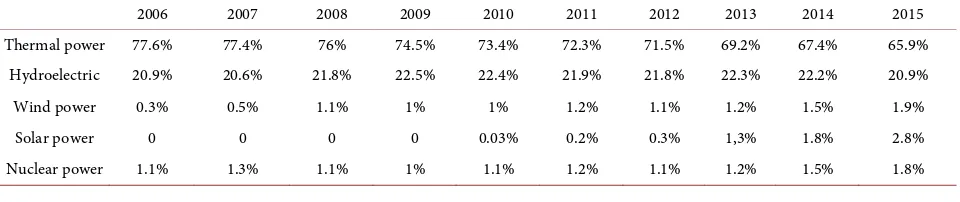
Chi-DOI: 10.4236/ajibm.2019.94065 952 American Journal of Industrial and Business Management na has long been a major energy consumer. And fossil fuels, especially coal, ac-count for a large proportion of China’s energy mix. In recent years, although the Chinese government has vigorously advocated the construction of “low-carbon economy”, the adjustment of energy structure still has a long way to go. In 2016, for example, coal still accounted for 61.83 percent of China’s energy mix, com-pared with 6.2 percent for natural gas, 2.82 percent for renewable energy and 8.62 percent for hydropower, according to the world energy statistics yearbook 2017. In the United States during the same period, coal accounted for only 15.77% and natural gas 31.52%. This is also closely related to China’s resource endowment of “rich coal, poor oil and little gas”. The energy structure of the electricity, thermal power production industry reflects the characteristics of China’s energy structure. The following table is compiled according to China statistical yearbook, which shows the proportion of each type of power genera-tion capacity in China from 2006 to 2015. From this, we can clearly see that the proportion of thermal power in the “eleventh five-year plan” and “twelfth five-year plan” period, although showing a downward trend year by year, but still occupies the dominant position. The production and industry of power and heat are still dominated by thermal power to provide kinetic energy for the de-velopment of national economy, which indicates the leading position of coal in the production input of this industry.
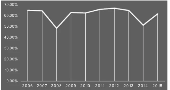
Table 1 shows that China’s energy structure is coal dependent. Such characte-ristics of the energy structure make China’s carbon emissions increase year by year. As early as 2007, China surpassed the United States as the world’s largest carbon dioxide emitter (Lee and Zhang [1]). Large increases in carbon emissions cause temperatures to rise, leading to water shortages, droughts and other severe weather. The energy structure dominated by fossil fuels has also caused serious damage to air quality in China. The six high-energy consuming industries dis-charge most of the carbon dioxide in our country. As one of the high-energy consuming industries, the production of electricity, thermal power production and supply industries uses coal as the main fuel, and is also the main consump-tion industry of coal energy, so they also emit a lot of carbon dioxide. Figure 1 shows that the amount of carbon dioxide emissions of electricity, thermal pro-duction and supply industry during the period of “eleventh five-year plan”, “twelfth five-year” has dominated the six energy-intensive industries more than a half of the total emissions (in addition to 2008, this paper argues that 2008
Table 1. The proportion of each type of power generation capacity.
2006 2007 2008 2009 2010 2011 2012 2013 2014 2015 Thermal power 77.6% 77.4% 76% 74.5% 73.4% 72.3% 71.5% 69.2% 67.4% 65.9%
Hydroelectric 20.9% 20.6% 21.8% 22.5% 22.4% 21.9% 21.8% 22.3% 22.2% 20.9% Wind power 0.3% 0.5% 1.1% 1% 1% 1.2% 1.1% 1.2% 1.5% 1.9%
DOI: 10.4236/ajibm.2019.94065 953 American Journal of Industrial and Business Management Figure 1. The amount of carbon dioxide emissions of electricity, thermal production and supply industry from 2006 to 2015.
Olympic Games country stepped up to the industry the management of pollu-tants discharge, slowed in 2008 emissions).
In addition to producing a lot of carbon dioxide, according to the 2009 China environmental statistical annual report, the power industry in this industry also emits a lot of nitrogen oxides and soot, accounting for 64.5% and 40.8% of the total national emissions in that year respectively. From this point of view, the pollutants produced by the production and supply industries of power and heat have an extremely important impact on the quality of China’s atmospheric en-vironment. The development of this industry is directly related to the improve-ment of air quality in China.
DOI: 10.4236/ajibm.2019.94065 954 American Journal of Industrial and Business Management development of the national economy. So it is necessary to analyze the efficiency of electricity, thermal power production and supply industries.
2. Literature Review
Distance function is a useful method to measure efficiency and productivity. Many scholars have applied it to different industries or enterprises. It differs from the traditional production function in that it can consider multiple inputs and outputs. In the efficiency analysis of industries (especially the polluting in-dustries), not only the good output but also the bad output should be taken into account, because some industries will produce a large number of pollutants in the production process. If not taken into account, the efficiency analysis will in-evitably be biased. The distance function can contain both good and bad outputs for efficiency analysis. It is the advantage that makes the distance function wide-ly used in the field of environmental economics. In essence, the distance func-tion can be regarded as a producfunc-tion funcfunc-tion composed of frontier. Specifically, the various production units which are regarded as research subject are facing a potential production frontier, this can also be called production technology boundaries. Input and output combination on the boundary of portfolio is the combination under the optimal condition. If production units are on the pro-duction boundary, we may consider the unit of propro-duction to be the most effi-cient, and the allocation of resources is also the most optimal condition. But in reality, the actual input-output combination of most production units is not an efficient combination, in other words, it deviates from the optimal technical boundary. At this time, there is a gap between the actual input-output tion of the inefficient production unit and the optimal input-output combina-tion, and the gap is the inefficiency level of the production unit, namely the es-timated value of the distance function, which is also the reason why this method is called the distance function. The distance function is divided into input dis-tance function, output disdis-tance function and direction disdis-tance function. The input distance function is input-oriented and assumes the same output, so as to calculate the minimum input that can be used to produce the same output. The output distance function is output oriented and measures the maximum output that the same input can produce. The directional distance function constructs a more demanding technology frontier, which requires the increase of good out-put and the decrease of bad outout-put.
DOI: 10.4236/ajibm.2019.94065 955 American Journal of Industrial and Business Management author used the traditional method to measure the efficiency and productivity of paper industry without considering the bad output. By comparing the two, the authors found that ignoring bad output understates firms’ performance, mainly because ignoring bad output ignores firms’ investment in cutting emissions. In the same way, Lee [6] evaluated the efficiency performance of 51 thermal power plants in the United States from 1977 to 1986, the shadow price of sulfur dioxide and the elasticity of substitution between sulfur dioxide and capital. The results show that the average efficiency of these thermal power plants is 0.945. Zhou et al. [7] adjusted the input distance function to keep the output, capital and labor unchanged, and then estimated the energy efficiency. The adjusted input dis-tance function is called the energy disdis-tance function. The energy disdis-tance func-tion is used to estimate the energy efficiency index of OECD countries based on SFA and non-parametric DEA. Lee and Zhang [1] applied the input distance function to 30 manufacturing industries in China for the first time, and eva-luated the technical efficiency of these industries. The results showed that seven industries were technically efficient, and the technical efficiency of printing in-dustry and copy inin-dustry of record media was only 0.26. Das and Kumbhakar [8], Das and Kumbhakar [9] studied the efficiency performance of Indian Banks based on the input distance function. Ma and Hailu [10] from 2001 to 2010, Chinese provincial data is used to estimate cost for the provinces of carbon emissions, this article will be three different distance functions are applied to the article has carried on the comparison and analysis, found that the output dis-tance function similar to the input disdis-tance function estimation results, direction distance function estimation results floating is bigger.
ana-DOI: 10.4236/ajibm.2019.94065 956 American Journal of Industrial and Business Management lyze the productivity changes of Irish dairy farms from 1984 to 2000. The result is that productivity on Ireland’s dairy farms is growing by 1.2% a year. Newman and Matthews [17] used the same method to compare the productivity of the four agricultural systems—sheep, cow pasture, farmland and cattle raising. Among them, the productivity of the sheep system increased the most, while that of the cattle raising system decreased. Feng and Serletis [18] studied the to-tal factor productivity of the large US Banks (assets at more than $one hundred million) from 2000 to 2005, and found that the average annual growth rate of these banks’ total factor productivity during this period is 1.98%, but the total factor productivity growth rate showed a trend of decline, this is mainly due to a slowdown in the technical improvement. Areal et al. [19] estimated the efficien-cy index of 215 dairy farms in England and wales based on the proportion of permanent pasture in total agricultural land as an environmental output based on the output distance function, and the results showed that the technical effi-ciency ranking of dairy farms changed after the addition of environmental out-put. Assaf and Agbola [20] calculate the efficiency value of accommodation in-dustry in Australia from 1998 to 2009, and found that different regions and dif-ferent types of accommodation departments have difdif-ferent efficiency scores, and considered that the degree of internationalization of regions, the proportion of large companies in the departments and the regional economic conditions were the main factors affecting the efficiency value.
DOI: 10.4236/ajibm.2019.94065 957 American Journal of Industrial and Business Management same time, the article results also indicated that a province’s industrial structure had a significant impact on the efficiency of its value. Murty et al. [25] used di-rection distance function to estimate the technical efficiency of India’s five pow-er and pollutant emission reduction cost. It is found that the avpow-erage technical efficiency of thermal power plants was 0.06, indicating that power has the poten-tial to improve the level of technology with 6% increase for good output and 6% reduction in pollution emissions at the same time, achieving output increased at the same time, but also improve environmental quality. Macpherson et al. [26] improved the traditional directional distance function in the calculation of the environmental performance of the United States region, and added more strin-gent requirements on the basis of the previous one, that is, the increase of good output and the decrease of bad output should be accompanied by the decrease of input. According to this theory, the author calculated the environmental tech-nology efficiency of 134 river basins on the east coast of the United States, and found that the evaluation of technology efficiency would be affected by the con-sideration of socio-economic factors, such as per capita national income and population density. Yuan et al. [27] studied the environmental efficiency of in-dustrial sector in 284 cities of China in 2003 and 2009, the average environmen-tal technology efficiency of China’s urban industrial sector is 0.947, of which the east has the highest efficiency value, followed in the west and in the middle of the lowest. The article further analyzed the factors that influence efficiency of environmental technology, and results showed that the U-shaped relationship is presented between income level and the technical efficiency. Foreign capital has played a positive role in the technical efficiency of ascension for industrial sec-tor, and denied the “pollution haven hypothesis”. Wang et al. [28] analyzed the energy efficiency and productivity of 28 provinces in China (excluding Hainan and Tibet) in the “eleventh five-year plan” by using the directional distance function, and compared three situations: energy conservation; energy conserva-tion and emission reducconserva-tion; energy conservaconserva-tion, emissions reducconserva-tion and economic growth. The study found that China’s energy efficiency and produc-tivity were very different in the three scenarios. In the third scenario, China’s energy efficiency during the 11th five-year plan period was 0.6306, while the av-erage annual growth rate of energy productivity was only 0.27%. Xie et al. [29] estimated the technical efficiency of each province, shadow price and the elastic-ity of substitution of the SO2 with industrial sector data of China’s 30 provinces
from 1998 to 2011 under the condition of considering the SO2 emissions. Results
showed that during the period of study, the technical inefficiency of China’s in-dustrial sector showed U-shaped curve change trend. And the turning point ap-peared in 2005. A positive elasticity of substitution between good and bad output suggests that a reduction in SO2 emissions is possible while boosting economic
growth.
DOI: 10.4236/ajibm.2019.94065 959 American Journal of Industrial and Business Management In this paper, the method of input distance function is used to estimate the ef-ficiency and productivity of electricity, thermal power production and supply industries in 30 provinces of China. On the basis of considering the regional he-terogeneity of the east, the middle and the west, this paper combines the meta-frontier with the input distance function to construct the metameta-frontier input distance function, and uses the two-stage parametric linear programming me-thod to estimate the distance function.
The structure of the rest of the paper is as follows. Section 2 introduces the metafrontier input distance function model we use to calculate the efficiency of the electricity, thermal power production and supply industries. Section 3 in-troduces the data in this paper. Section 4 is empirical results analysis. Section 5 summarizes the research conclusion and puts forward the policy suggestions.
3. Methodology
3.1. The Metafrontier Input Distance Function
We assume a production unit which produces good output and bad output. This production unit’s inputs are g
(
, ,)
t
x = l k e , outputs are g
( )
,t
y = q u . L, k and e represent labor, capital and energy respectively. q and u denote good output and bad output respectively. In this paper, good output is defined as the total indus-trial output of the power, thermal power production and supply industry, while bad output is defined as the carbon dioxide emissions of the industry. Super-script g and the subscript t are group and time respectively. According to She-phard [3], the input distance function is:
(
g, g)
sup 0 : tg( )
gg g
t x yt t x t yt
D θ F
θ
= ∈
(1)
In the model (1), F ytg
( )
tg represents the demand set of input factors. TheDOI: 10.4236/ajibm.2019.94065 960 American Journal of Industrial and Business Management Since the value of the input distance function g
(
g, g)
t t
t x
D y is the ratio be-tween the actual input and potential input for the production unit, we can use the inverse of the input distance function to express the technical efficiency of the production unit according to Farrell [43]:
(
1)
(
)
0 , 1
,
g g g
t t t
g g g
t t t
TE x y D x y
≤ = ≤ (2)
As discussed above in the common boundary section, economic environment, regional differences, policy factors, etc., will cause each production unit within the technical boundary to form a group (for example, the east and west three groups in this paper), so a common boundary must be constructed to measure the production potential of each production unit. This technical boundary means the potential optimal portfolio of inputs that can be achieved when dif-ferences between each group converge. We define the input distance function of the common boundary as:
(
,)
sup 0 :( )
m t m
t t t x t t
D x y θ F y
θ
= ∈
(3)
( )
mt t
F y is the demand set of input factors based on common boundary. The boundary of the set is the common boundary. Common boundaries mean that production units have greater potential to reduce inputs than intra-group tech-nical boundaries.
Similar to formula (2), the reciprocal of the input distance function value of the common boundary is used to express the technical efficiency based on the common boundary:
(
,)
(
)
1 , 1
0 t t
t t m t m t x y x y TE D
≤ = ≤ (4)
By combining formula (2) and formula (4), we can calculate the technical gap t TGR:
(
)
(
)
(
(
)
)
, , , , t t t tg g g m
t t t t
t m g g g
t t t t
D x y TE
TGR
D T
y
x y E x
x y
= = (5)
3.2. Parametric Linear Programming
DOI: 10.4236/ajibm.2019.94065 961 American Journal of Industrial and Business Management 3.2.1. Functional Form
Parametric linear programming begins with selecting the appropriate functional form to simulate the technical boundary. According to Christensen et al. [44], Hailu and Veeman [5] applied the transcendental logarithm function to the esti-mation of input distance function, and the flexibility of this function can well simulate the technical boundary of input orientation. Taking the intra-group distance function as an example, the transcendental logarithm function is ex-pressed as:
(
)
0 , ,, , , ,
2
, , , ,
ln , , ln ln
1 ln ln 1 ln ln
2 2
1 ln ln ln ln
2
hg g g g g
t t t i i t j j t
i j
g g g g
ii i t i t jj j t j t
i i j j
g g g g
i i t j j t ij i t j t
i j i j
D x y t x y t
x x y y
t x t y t x y
α α β χ
ε φ
δ ϕ γ ο
′ ′ ′ ′ ′ ′ = + + + + + + + + +
∑
∑
∑∑
∑∑
∑
∑
∑∑
(6)In formula (6), superscript h represents the number of research objects. The lowercase letter g indicates that the function corresponds to the inner group boundary. i i, ′ denotes inputs (k, e, l). j j, ′ indicates outputs (q, u). α α β0, ,i j and so on are parameters to be estimated. The functional form of the common boundary is the same as that of Equation (6), which will not be repeated here. 3.2.2. The Estimation of Intragroup
Aigner and Chu [45] firstly used the method of linear programming for parame-ter estimation. Hailu and Veeman [5] used parametric linear programming to es-timate the value of the input distance function. Parametric linear programming is very flexible, and it is convenient to apply various constraints on the distance function so as to better simulate the technical boundary of input guidance. Therefore, from this perspective, it is more suitable for estimating the input dis-tance function than the econometric method. The parametric linear program-ming problem based on the inner boundary of the group is expressed as follows:
(
)
( )
(
)
( )
(
)
( )
(
)
min ln , , ln1
s.t. 1 ln , , 0,
ln , ,
2 0,
ln
ln , ,
3 0,
ln
hg g g
t t t
h
g g g
t t t
g g g
t t t
g t
g g g
t t t
g t
D x y t
D x y t D x y t
q D x y t
u − ≥ ∂ ≤ ∂ ∂ ≥ ∂
∑
( )
(
)
( )
( )
( )
ln , ,
4 0,
ln
5 1,
6 0,
7 ,
g g g
t t t
g t
i i
ii ij i
i i i
ii i i jj j j
D x y t x
α
ε ο ϕ
ε ε φ φ
DOI: 10.4236/ajibm.2019.94065 962 American Journal of Industrial and Business Management Formula (7) is essentially a goal minimization problem, that is, to make the actual input portfolio approach the potential input portfolio. Constraint condi-tion (1) limits the value range of the input distance funccondi-tion. The value of the input distance function is greater than or equal to 1, which indicates that the ac-tual input has potential to reduce. (2), (3) and (4) indicate the monotonicity of the input distance function on good output, bad output and input. (5) and (6) constrain the homogeneity of the function with respect to input. (7) is a con-straint on symmetry.
3.2.3. The Estimation of Metafrontier
Formula (7) shows the parametric linear programming of the inner boundary of the group. The estimation of the parametric linear programming of the common boundary is as follows:
(
)
(
)
( )
(
)
(
)
( )
(
)
( )
(
)
min ln , , ln , ,
s.t. 1 ln , , ln , , ,
ln , ,
2 0,
ln
ln , ,
3 0,
ln
hm m m g g g
t t t t t t
h
m m m g g g
t t t t t t
m m m
t t t
m t
m m m
t t t
m t
D x y t D x y t
D x y t D x y t
D x y t q D x y t
u − ≥ ∂ ≤ ∂ ∂ ≥ ∂
∑
( )
(
)
( )
( )
( )
ln , ,
4 0,
ln
5 1,
6 0,
7 ,
m m m
t t t
m t
i i
ii ij i
i i i
ii i i jj j j
D x y t x
α
ε ο ϕ
ε ε φ φ
′ ′ ′ ′ ′ ∂ ≥ ∂ = = = = = =
∑
∑
∑
∑
(8)It should be noted that the objective function and constraint condition (1) of the above formula are different from that of (7), because the common boundary must cover the inner boundary of the group and be as close as possible to it. The following figure illustrates this idea.
4. Data
DOI: 10.4236/ajibm.2019.94065 963 American Journal of Industrial and Business Management value by PPI on the basis of unchanged price in 2006, and the carbon dioxide emissions came from CEADs database. In terms of the calculation of capital stock, this paper, takes the average annual balance of the net fixed assets as the capital stock. Labor is the total number of annual employees in the power, heat and supply industries in each province. Energy input is expressed as standard coal (converted into standard coal in proportion to various energy sources). De-scriptive statistics of all data are shown in Table 2.
[image:14.595.205.539.416.732.2]As shown in the table below, the national data are grouped by east, middle and west. There are 14 provinces in the east, including Anhui, Beijing, Fujian, Guangdong, Hainan, Hebei, Heilongjiang, Jilin, Jiangsu, Liaoning, Shandong, Shanghai, Tianjin and Zhejiang. There are six central provinces, namely, Henan, Hunan, Hubei, Jiangxi, Inner Mongolia and Shanxi. There are 10 western prov-inces: Gansu, Guangxi, Guizhou, Ningxia, Qinghai, Shaanxi, Sichuan, Xinjiang, Yunnan and Chongqing. It can be seen from the table that the input-output of the three groups shows some differences. Among them, the average output value of the eastern power and thermal power production and supply industries is the highest, followed by the central region and the lowest in the western region. This is because the eastern regions are economically developed and densely popu-lated, so the demand for electricity and heat is much higher than that in the cen-tral and western regions. At the same time, the eastern region has the most ad-vanced productivity. We can see that the eastern region and the central region
Table 2. The description of data.
Group Variable Unit Observation Mean S.D. Min Max q billion 140 1113.79 815.90 65.79 3378.15 u 104 ton 140 15,843.89 10,957.44 820.62 45,390
East k billion 140 1113.25 727.95 102.58 3163.40 e Standard coal 104 ton 140 1749.75 1170.69 52.54 4182.77 l 104 person 140 9.55 5.71 1.17 23.24
q billion 60 740.97 380.20 361.57 1766.58 u 104 ton 60 17,459.83 10,212.42 4620.67 42,009
Middle k billion 60 1227.23 665.02 374.65 2574.73 e Standard coal 104 ton 60 1705.27 617.22 557.57 3089.09 l 104 person 60 11.11 3.80 5.14 20.62
q billion 100 341.15 181.05 91.12 690.14 u 104 ton 100 7204.80 3674.29 970.76 21100
DOI: 10.4236/ajibm.2019.94065 964 American Journal of Industrial and Business Management do not have much difference in input, but the eastern region has a higher output value. The eastern and central regions use a lot of energy, so these two regions are the major CO2 emitters.
In order to prove the rationality of our grouping, we used the nonparametric K-W rank sum test to test the results of mixed estimation according to the test method of Casu et al. (2013). The difference between mixed estimation and common boundary based estimation is that it assumes that there is no group difference among all production units. In this paper, the mixed estimation is to estimate all the data of 30 provinces with not considering the grouping. We ap-plied the estimated results of this method to the K-W test, and the results shows that the P value is 0.0310, so the null hypothesis is rejected at the significance level of 5%, which indicated that it is very necessary for us to divide the national data into three groups, and the mixed estimation would produce deviation on the efficiency estimation.
5. Empirical Analysis
5.1. The Estimation of Parameters
[image:15.595.201.540.451.729.2]In this section, we combine the data used with the common boundary distance function model to obtain the efficiency of electricity, thermal power production and supply industries in 30 provinces of China. We use GAMS software to esti-mate the transcendental logarithm function to obtain the values of each coeffi-cient. In order to make the results converge, we standardized the data in the es-timation. Table 3 shows the results of the coefficient estimation.
Table 3. The estimation of parameters for metafrontier input distance function.
Parameter Variable East Middle West Metafrontier
0
α intercept 0.1608 0.1515 0.4736 0.3601
k
α lnxk 0.8043 0.5444 0.6612 0.7042 e
α lnxe 0.1436 0.0556 0.3316 0.1951 l
α lnxl 0.0521 0.4000 0.0072 0.1007 q
β lnyq −1.0033 −1.2217 −1.1694 −0.9675 u
β lnyu 0.0159 0.4840 0.2980 0.0226
χ t −0.0098 −0.0195 −0.0576 −0.0130
kk
ε lnxk⋅lnxk −0.9093 −1.2344 −0.9353 −0.5562 ke
ε lnxk⋅lnxe 0.0544 0.1392 0.5842 0.0853 kl
ε lnxk⋅lnxl 0.3861 0.2162 0.0332 0.1873 ek
ε lnxe⋅lnxk 0.0544 0.1392 0.5842 0.0853 ee
ε lnxe⋅lnxe 0.0057 −0.0937 −0.2855 0.0158 el
ε lnxe⋅lnxl 0.0190 0.1936 −0.0006 0.0193 lk
ε lnxl⋅lnxk 0.3861 0.2162 0.0332 0.1873 le
DOI: 10.4236/ajibm.2019.94065 965 American Journal of Industrial and Business Management
Continued
ll
ε lnxl⋅lnxl −0.0154 0.2301 −0.0130 −0.0435 qq
φ lnyq⋅lnyq −0.0702 0.8191 −0.1761 −0.1154 qu
φ lnyq⋅lnyu 0.0009 0.9495 0.3815 0.0422 uq
φ lnyu⋅lnyq 0.0009 0.9495 0.3815 0.0422 uu
φ lnyu⋅lnyu 0.0119 −0.0306 −0.2640 0.0006
δ t2 0.0014 0.0015 0.0057 0.0022
k
ϕ lnx tk⋅ 0.0112 0.0105 0.0059 0.0121 e
ϕ lnx te⋅ −0.0113 0.0077 −0.0061 −0.0148 l
ϕ lnx tl⋅ 0.0001 −0.0182 0.0002 0.0027 q
γ lny tq⋅ −0.0014 −0.0019 0.0393 −0.0041 u
γ lny tu⋅ 0.0008 −0.0312 −0.0148 0.0039 kq
ο lnxk⋅lnyq 0.4544 0.8529 0.5347 0.3511 ku
ο lnxk⋅lnyu 0.0175 −0.4130 −0.5123 −0.0259 eq
ο lnxe⋅lnyq −0.0259 −0.2603 −0.1804 −0.0944 eu
ο lnxe⋅lnyu −0.0486 0.0930 0.1746 −0.0304 lq
ο lnxl⋅lnyq −0.3917 −0.2868 −0.0154 −0.2226 lu
ο lnxl⋅lnyu −0.0056 0.0142 −0.0012 0.0222
5.2. The Efficiency Analysis of Electricity, Thermal Power
Production and Supply Industry
[image:16.595.211.539.85.364.2]5.2.1. Description of Various Efficiency Indicators in the East, Middle and West
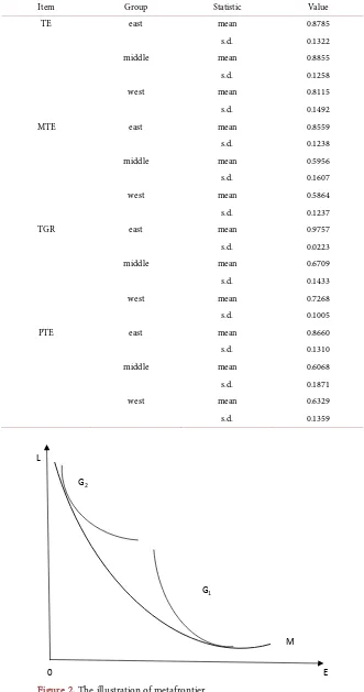
Table 4 shows the technical efficiency and technical gap between the electricity, thermal power production and supply industries in the east, middle and west. In the Table 4, PTE is the efficiency value calculated by using mixed estimation, and the results are listed for the purpose of comparing with the result of meta-frontier estimation. TE stands for technical efficiency based on intra group boundaries. MTE is the result of metafrontier estimation. TGR is the quotient between MTE and TE, indicating the technical gap. Table 4 is described in three aspects below.
DOI: 10.4236/ajibm.2019.94065 966 American Journal of Industrial and Business Management Table 4. Estimation of efficiency.
Item Group Statistic Value
TE east mean 0.8785
s.d. 0.1322 middle mean 0.8855 s.d. 0.1258 west mean 0.8115 s.d. 0.1492
MTE east mean 0.8559
s.d. 0.1238 middle mean 0.5956 s.d. 0.1607 west mean 0.5864 s.d. 0.1237
TGR east mean 0.9757
s.d. 0.0223 middle mean 0.6709 s.d. 0.1433 west mean 0.7268 s.d. 0.1005
PTE east mean 0.8660
[image:17.595.208.539.91.720.2]s.d. 0.1310 middle mean 0.6068 s.d. 0.1871 west mean 0.6329 s.d. 0.1359
Figure 2. The illustration of metafrontier.
G2
G1
M L
DOI: 10.4236/ajibm.2019.94065 967 American Journal of Industrial and Business Management Secondly, in terms of TE, the performance of the east and the middle is not different, but the efficiency value in the west is significantly lower than that in the east and the middle. Such results cannot indicate which of the east, west and east regions performs better in efficiency, because the TE value is only compared within each region. Only the value of MTE can truly reflect the efficiency differ-ence between east, middle and west, because they are all compared based on a common boundary (metafrontier) at this time. Table 4 shows that the MTE value in the east is much higher than that in the Middle and west, while that in the middle is slightly higher than that in the west. This indicates that the eastern region is significantly more efficient if the common potential technology boun-dary is used as the benchmark. Because the economic and technological level of the east is stronger than that of the central and western regions, the eastern re-gion as a whole is closer to the potential technological boundary. It also means that for the same amount of output, the east can do it with less input. The dif-ference in MTE between the east and the middle can also explain why the input used is similar but the output value in the east is higher (Table 2).
Finally, we analyze the technical gap (TGR). TGR reflects the gap between in-tra group frontier and metafrontier. Clearly, the TGR performance in the east is much better than that in the middle and west. It shows again that the input portfolio of eastern power, thermal power production and supply industries is closer to the potential optimal input portfolio. In addition, TGR is 0.6709 in the middle and 0.7268 in the west. The reason why the middle part is smaller than the west part is that TGR is the quotient of MTE and TE. Although the TE in the middle part is higher than that in the west part, the MTE of the two is not much different, which ultimately makes the TGR in the west higher than that in the middle part.
On the whole, in the electricity, thermal power production and supply indus-tries, the efficiency performance of the eastern region is better than that of the central and western regions, showing an unbalanced state of development. The central and western regions need to improve technology, further optimize the investment mix, and get rid of the extensive development mode.
5.2.2. The Trending Analysis of Efficiency for 30 Provinces
Next, we will analyze the annual change trend of TE, MTE and TGR in the east-ern, central and western regions. Figures 3-5 respectively show the trend change charts of the three indicators during the “eleventh five-year plan” and “twelfth five-year plan”.
DOI: 10.4236/ajibm.2019.94065 968 American Journal of Industrial and Business Management Figure 3. The trending of efficiency based on intragroup frontier.
Figure 4. The trending of efficiency based on metafrontier.
[image:19.595.213.538.520.706.2]DOI: 10.4236/ajibm.2019.94065 969 American Journal of Industrial and Business Management and gradually leveled off from 2013 to 2015. Secondly, the technical efficiency of the electricity, thermal power production and supply industry in the central re-gion shows a trend of decreasing at first and then increasing, with a large range of change. With 2011 as the turning point, it was on a downward trend before and then on an upward trend. Finally, the efficiency performance of the western region was relatively stable before 2012, during which there were rises and falls, but the range was small, and then it showed an obvious upward trend until 2015. To sum up, the technical efficiency of the eastern region showed a stable trend during the “eleventh five-year plan” and “twelfth five-year plan”, with an overall slight increase. The technical efficiency within the group in the central and western regions showed obvious differences during the “eleventh five-year plan” and “twelfth five-year plan”. This paper believes that the rising of the two in the “twelfth five-year plan” is mainly due to the gradual slowing of China’s econom-ic growth during this period, wheconom-ich has entered the new normal, and the country pays more attention to the development of economic quality. These changes will force the electricity, thermal power production and supply industries to improve technology and efficiency in the production process.
We use Figure 3 and Figure 4 to compare the efficiency performance of east and west based on metafrontier. From the two figures, it is clear that the electric-ity, thermal power production and supply industries in the east is more techni-cally efficient than that in the middle and west based on metafrontier. Moreover, the central and western regions did not show a catch-up trend during the 11th and 12th five-year plans. This situation shows that the east, the central and western regions appear unbalanced state of development. The east as a whole is closer to the common boundary (metafrontier), representing the most advanced level of development in China’s electricity, thermal power production and supply industries. However, there is still a big gap between three regions. Al-though their intra-group technical efficiency has been greatly improved during the “twelfth five-year plan” period, their actual input portfolio is still far from the potential optimal input portfolio, and there is no substantial progress during the whole “eleventh five-year plan” and “twelfth five-year plan” period. There-fore, the electricity, thermal power production and supply industries in the cen-tral and western regions still have much room for improvement in optimizing the investment mix.
6. Summary and Conclusion
DOI: 10.4236/ajibm.2019.94065 970 American Journal of Industrial and Business Management that in the middle and west, that is, the east is closer to the potential production boundary. During the 11th and 12th five-year plans, the gap between the central, western regions and the eastern regions did not shrink. Therefore, we can think that the development of China’s power, thermal power production and supply industry is unbalanced. In the future, the state should actively change the devel-opment mode of electricity, thermal power production and supply industries in the central and western regions, and take a series of measures to improve the level of technology and productivity in the central and western regions.
This paper mainly analyzes the efficiency performance of electricity, thermal power production and supply industries. Efficiency analysis is only a static anal-ysis, so it can further analyze the change of dynamic productivity in the industry in the future. In addition, due to the linear programming method used in this paper, the estimation results lack relevant statistics. In future research, bootstrap method can be used to solve this problem.
Conflicts of Interest
The author declares no conflicts of interest regarding the publication of this pa-per.
References
[1] Lee, M. and Zhang, N. (2012) Technical Efficiency, Shadow Price of Carbon Dio-xide Emissions, and Substitutability for Energy in the Chinese Manufacturing In-dustries. Energy Economics, 34, 1492-1497.
https://doi.org/10.1016/j.eneco.2012.06.023
[2] Shephard, R.W. (1953) Cost and Production Function. Princeton University Press, Princeton.
[3] Shephard, R.W. (1970) Theory of Cost and Production Function. Princeton Univer-sity Press, Princeton.
[4] Färe, R. and Primont, D. (1995) Multi-Output Production and Duality: Theory and Application. Kluwer Academic Publishers, Boston.
https://doi.org/10.1007/978-94-011-0651-1
[5] Hailu, A. and Veeman, T.S. (2000) Environmentally Sensitive Productivity Analysis of the Canadian Pulp and Paper Industry, 1959-1994: An Input Distance Function Approach. Journal of Environmental Economics & Management, 40, 251-274.
https://doi.org/10.1006/jeem.2000.1124
[6] Lee, M. (2005) The Shadow Price of Substitutable Sulfur in the US Electric Power Plant: A Distance Function Approach. Journal of Environmental Management, 77, 104-110. https://doi.org/10.1016/j.jenvman.2005.02.013
[7] Zhou, P., Ang, B.W. and Zhou, D.Q. (2012) Measuring Economy-Wide Energy Effi-ciency Performance: A Parametric Frontier Approach. Applied Energy, 90, 196-200.
https://doi.org/10.1016/j.apenergy.2011.02.025
[8] Das, A. and Kumbhakar, S.C. (2012) Productivity and Efficiency Dynamics in dian Banking: An Input Distance Function Approach Incorporating Quality of In-puts and OutIn-puts. Journal of Applied Econometrics, 27, 205-234.
https://doi.org/10.1002/jae.1183
DOI: 10.4236/ajibm.2019.94065 971 American Journal of Industrial and Business Management
Input Distance Function Approach. Empirical Economics, 51, 1689-1719
https://doi.org/10.1007/s00181-015-1062-4
[10] Ma, C.B. and Hailu, A. (2016) The Marginal Abatement Cost of Carbon Emissions in China. The Energy Journal, 37, 111-127.
https://doi.org/10.5547/01956574.37.si1.cma
[11] Färe, R., Grosskopf, S., Lovell, C.A.K. and Pasurka, C.A. (1989) Multilateral Prod-uctivity Comparison when Some Outputs Are Undesirable: A Nonparametric Ap-proach. Review of Economics and Statistics, 71, 90-98.
https://doi.org/10.2307/1928055
[12] Färe, R., Grosskopf, S., Lovell, C.A.K. and Yaisawarng, S. (1993) Derivation of Sha-dow Prices for Undesirable Outputs: A Distance Function Approach. Review of Economics and Statistics, 75, 374-380. https://doi.org/10.2307/2109448
[13] Coggins, J.S. and Swinton J.R. (1996) The Price of Pollution: A Dual Approach to Valuing SO2 Allowances. Journal of Environmental Economics and Management,
30, 58-72. https://doi.org/10.1006/jeem.1996.0005
[14] Swinton, J.R. (1998) At What Cost Do We Reduce Pollution? Shadow Prices of SO2
Reduction. The Energy Journal, 19, 63-83.
https://doi.org/10.5547/issn0195-6574-ej-vol19-no4-3
[15] Swinton, J.R. (2002) The Potential for Cost Savings in the Sulfur Dioxide Allowance Market: Empirical Evidence from Florida. Land Economics, 78, 390-404.
https://doi.org/10.2307/3146897
[16] Newman, C. and Matthews, A. (2006) The Productivity Performance of Irish Dairy Farms 1984-2000: A Multiple Output Distance Function Approach. Journal of Productivity Analysis, 26, 191-205. https://doi.org/10.1007/s11123-006-0013-7
[17] Newman, C. and Matthews, A. (2007) Evaluating the Productivity Performance of Agricultural Enterprises in Ireland Using a Multiple Output Distance Function Ap-proach. Journal of Agricultural Economics, 58, 128-151.
https://doi.org/10.1111/j.1477-9552.2007.00084.x
[18] Feng, G. and Serletis, A. (2010) Efficiency, Technical Change, and Returns to Scale in Large US Banks: Panel Data Evidence from an Output Distance Function Satis-fying Theoretical Regularity. Journal of Banking & Finance, 34, 127-138.
https://doi.org/10.1016/j.jbankfin.2009.07.009
[19] Areal, F.J., Tiffin, R. and Balcombe, K.G. (2012) Provision of Environmental Output within a Multi-Output Distance Function Approach. Ecological Economics, 78, 47-54. https://doi.org/10.1016/j.ecolecon.2012.03.011
[20] Assaf, A.G. and Agbola, F.W. (2012) Efficiency Analysis of the Australian Accom-modation Industry: A Bayesian Output Distance Function. Journal of Hospitality & Tourism Research, 38, 116-132. https://doi.org/10.1177/1096348012451459
[21] Chung, Y.H., Färe, R. and Grosskopf, S. (1997) Productivity and Undesirable Out-puts: A Directional Distance Function Approach. Journal of Environmental Man-agement, 51, 229-240. https://doi.org/10.1006/jema.1997.0146
[22] Färe, R., Grosskopf, S., Noh, D.W. and Weber, W. (2005) Characteristics of a Pol-luting Technology: Theory and Practice. Journal of Econometrics, 126, 469-492.
https://doi.org/10.1016/j.jeconom.2004.05.010
[23] Mcmullen, B.S. and Noh, D.W. (2007) Accounting for Emissions in the Measure-ment of Transit Agency Efficiency: A Directional Distance Function Approach.
Transportation Research, Part D: Transport and Environment, 12, 1-9.
DOI: 10.4236/ajibm.2019.94065 972 American Journal of Industrial and Business Management
[24] Watanabe, M. and Tanaka, K. (2007) Efficiency Analysis of Chinese Industry: A Directional Distance Function Approach. Energy Policy, 35, 6323-6331.
https://doi.org/10.1016/j.enpol.2007.07.013
[25] Murty, M.N., Kumar, S. and Dhavala, K.K. (2007) Measuring Environmental Effi-ciency of Industry: A Case Study of Thermal Power Generation in India. Environ-mental and Resource Economics, 38, 31-50.
https://doi.org/10.1007/s10640-006-9055-6
[26] Macpherson, A.J., Principe, P.P. and Smith, E.R. (2010) A Directional Distance Function Approach to Regional Environmental-Economic Assessments. Ecological Economics, 69, 1918-1925. https://doi.org/10.1016/j.ecolecon.2010.04.012
[27] Yuan, P., Cheng, S., Sun, J. and Liang, W.B. (2013) Measuring the Environmental Efficiency of the Chinese Industrial Sector: A Directional Distance Function Ap-proach. Mathematical and Computer Modelling, 58, 936-947.
https://doi.org/10.1016/j.mcm.2012.10.024
[28] Wang, H., Zhou, P. and Zhou, D.Q. (2013) Scenario-Based Energy Efficiency and Productivity in China: A Non-Radial Directional Distance Function Analysis.
Energy Economics, 40, 795-803. https://doi.org/10.1016/j.eneco.2013.09.030
[29] Xie, H., Shen, M. and Wei, C. (2016) Technical Efficiency, Shadow Price and Subs-titutability of Chinese Industrial SO2 Emissions: A Parametric Approach. Journal of
Cleaner Production, 112, 1386-1394. https://doi.org/10.1016/j.jclepro.2015.04.122
[30] Hayami, Y. (1969) Sources of Agricultural Productivity Gap among Selected Coun-tries. American Journal of Agricultural Economics, 51, 564-575.
https://doi.org/10.2307/1237909
[31] Hayami, Y. and Ruttan, V.W. (1970) Agricultural Productivity Differences among Countries. American Economic Review, 60, 895-911.
[32] Battese, G.E. and Rao, D.S.P. (2002) Technology Gap, Efficiency, and a Stochastic Metafrontier Function. International Journal of Business and Economics, 1, 87-93. [33] Rao, D.S.P., O’Donnell, J.C. and Battese, G.E. (2003) Metafrontier Functions for the
study of Inter-Regional Productivity Differences. Center for Efficiency and Produc-tivity Analysis, Working Paper.
[34] Battese, G.E., Rao, D.S.P. and O’Donnell, J.C. (2004) A Metafrontier Production Function for Estimation of Technical Efficiencies and Technology Gaps for Firms Operating under Different Technologies. Journal of Productivity Analysis, 21, 91-103. https://doi.org/10.1023/b:prod.0000012454.06094.29
[35] O’Donnell, Rao, D.S.P., J.C. and Battese, G.E. (2008) Metafrontier Frameworks for the Study of Firm-Level Efficiencies and Technology Ratios. Empirical Economics, 34, 231-255. https://doi.org/10.1007/s00181-007-0119-4
[36] Huang, Y.J., Chen, K.H. and Yang, C.H. (2010) Cost Efficiency and Optimal Scale of Electricity Distribution Firms in Taiwan: An Application of Metafrontier Analysis.
Energy Economics, 32, 15-23. https://doi.org/10.1016/j.eneco.2009.03.005
[37] Chen, K.H. (2012) Incorporating Risk Input into the Analysis of Bank Productivity: Application to the Taiwanese Banking Industry. Journal of Banking & Finance, 36, 1911-1927. https://doi.org/10.1016/j.jbankfin.2012.02.012
[38] Huang, C.J., Huang, T.H. and Liu, N.H. (2014) A New Approach to Estimating the Metafrontier Production Function Based on a Stochastic Frontier Framework.
Journal of Productivity Analysis, 42, 241-254.
https://doi.org/10.1007/s11123-014-0402-2
DOI: 10.4236/ajibm.2019.94065 973 American Journal of Industrial and Business Management
Directional Distance Function to Compare Banking Efficiencies in Central and Eastern European Countries. Economic Modelling, 44, 188-199.
https://doi.org/10.1016/j.econmod.2014.10.029
[40] Zhang, N. and Wang, B. (2015) A Deterministic Parametric Metafrontier Luen-berger Indicator for Measuring Environmentally-Sensitive Productivity Growth: A Korean Fossil-Fuel Power Case. Energy Economics, 51, 88-98.
https://doi.org/10.1016/j.eneco.2015.06.003
[41] Du, L.M., Hanley, A. and Zhang, N. (2016) Environmental Technical Efficiency, Technology Gap and Shadow Price of Coal-Fuelled Power Plants in China: A Para-metric Meta-Frontier Analysis. Resource and Energy Economics, 43, 14-32.
https://doi.org/10.1016/j.reseneeco.2015.11.001
[42] Färe, R. and Grosskopf, S. (1990) A Distance Function Approach to Price Efficiency.
Journal of Public Economics, 43, 123-126.
https://doi.org/10.1016/0047-2727(90)90054-l
[43] Farrell, M.J. (1957) The Measurement of Productive Efficiency. Journal of the Royal Statistical Society, 120, 253-281.
[44] Christensen, L.R. and Lau, J.L.J. (1973) Transcendental Logarithmic Production Frontiers. The Review of Economics and Statistics, 55, 28-45.
[45] Aigner, D.J. and Chu, S.F. (1968) On Estimating the Industry Production Function.