1 1
Title: Quantification of Drought During the Collapse of the Classic Maya
2Civilization
34
Authors: Nicholas P. Evans1*, Thomas K. Bauska1, Fernando Gázquez1, Mark 5
Brenner2, Jason H. Curtis2, and David A. Hodell1 6
Affiliations:
7
1Godwin Laboratory for Palaeoclimate Research, Department of Earth Sciences,
8
University of Cambridge, Downing Street, Cambridge, CB2 3EQ, United Kingdom. 9
2Department of Geological Sciences, University of Florida, Gainesville, FL 32611,
10
USA. 11
2
Abstract: 13
14
The demise of Lowland Classic Maya civilization during the Terminal Classic Period 15
(~800-1000 C.E.) is a well-cited example of how past climate may have impacted 16
ancient societies. Attempts to estimate the magnitude of hydrologic change, however, 17
have met with equivocal success because of the qualitative and indirect nature of 18
available climate proxy data. We reconstructed the past isotopic composition (δ18O, 19
δD, 17O-excess and d-excess) of water in Lake Chichancanab, Mexico, using a novel 20
technique that involves isotopic analysis of the structurally bound water in 21
sedimentary gypsum, which was deposited under drought conditions. The triple 22
oxygen and hydrogen isotope data provide a direct measure of past changes in lake 23
hydrology. We modeled the data and conclude that annual precipitation decreased 24
between 41 and 54%, with intervals of up to 70% rainfall reduction during peak 25
drought conditions, and relative humidity declined by 2 to 7% compared to today.
26 27
One Sentence Summary:
28 29
We present quantitative estimates of hydro-climate changes that coincided with the 30
demise of the Classic Maya civilization. 31
32
Main Text:
33 34
More than two decades ago, a sediment core from Lake Chichancanab 35
(Yucatán Peninsula, Mexico; Fig. S1) provided the first physical evidence of a 36
temporal correlation between drought and the sociopolitical transformation of the 37
Classic Maya civilization during the Terminal Classic Period (TCP) (1). Presence of 38
gypsum horizons and a concomitant increase in the oxygen isotope ratio (18O/16O) in 39
shells of ostracods and gastropods suggested the TCP was among the driest periods of 40
the Holocene in northern Yucatán. Paleoclimate records produced subsequently 41
provided additional evidence for drought during the TCP (2-9), but the magnitude of 42
hydro-climate change and its influence on Maya agricultural and sociopolitical 43
3 archives, combined with dating uncertainties, has prevented detailed assessment of 45
the relationship between past climate and cultural changes (10-12). 46
47
Recent attempts to quantify estimates of past changes in rainfall amount and 48
assess the impact on ancient Maya agriculture have utilized either oxygen (δ18O) (6,
49
13) or hydrogen (δD) (9-11) isotopes. No study to date has combined the two isotope 50
systems because materials used for analysis, e.g., carbonates and leaf waxes, preclude 51
simultaneous measurement of the multiple isotopologues of water. Combined analysis 52
of δ18O, δ17O and δD is a powerful method to estimate past hydrologic changes 53
quantitatively because hydrogen and triple oxygen isotopes each undergo slightly 54
different fractionation during evaporation, leading to changes in the derived d-excess 55
(δD – 8 ·δ18O) and 17O-excess (ln[δ17O + 1] − 0.528 ln[δ18O +1]) parameters (14-19). 56
In an effectively closed hydrological basin such as Lake Chichancanab, the primary 57
controls on the isotopic fractionation of lake water during evaporation include: the 58
fractional loss of precipitation to evaporation (P/E), normalized relative humidity 59
(RHn), temperature, and changes in the precipitation source (1-3, 14). The d-excess is
60
largely dependent on RHn and temperature, whereas 17O-excess is controlled mainly
61
by RHn (14-19). Because the predicted trends of d-excess and 17O-excess in
62
evaporating waters display different responses to climate variables, they can be 63
evaluated individually using an iterative model (20). 64
65
We took advantage of the benefits of using all isotopologues of water and their 66
derived parameters (d-excess and 17O-excess) by measuring triple oxygen and
67
hydrogen isotopes in the hydration water of gypsum (CaSO4·2H2O) in sediment cores
68
from Lake Chichancanab (Fig. S2) (3). Today, the lake water is near saturation for 69
gypsum and during past periods of drier climate, when the lake volume shrank, 70
gypsum precipitated from the lake water and was preserved as distinct layers within 71
the accumulating sediments (1-3). When gypsum forms, water molecules are 72
incorporated directly into its crystalline structure and this “gypsum hydration water” 73
(GHW) records the isotopic composition of the parent fluid, with known isotopic 74
fractionations (14, 17, 21-26). Unlike oxygen isotope fractionation during formation 75
4 practically independent of temperature (24), biological or kinetic (non-equilibrium) 77
effects (17). Additionally, isotopes of GHW that are measured in the sedimented 78
gypsum inherently record the driest periods, offering a distinct advantage over other 79
traditional climate archives such as speleothems or mollusk shells, which may fail to 80
register peak drought conditions because of growth hiatuses. Absolute differences in 81
the δ18O, δD, 17O-excess and d-excess, between modern and paleo-lake water, provide 82
an estimate of differences between the lake hydrologic budget during the TCP and 83
today (Fig. 1). Results were evaluated using a numerical isotope mass balance model 84
that must satisfy all isotope variables (20) (Fig. S3), and thus provides a more robust 85
constraint on past hydrology than does modeling δ18O or δD alone. 86
87
The modern climate around Lake Chichancanab is characterized by a mean 88
annual precipitation of ~1200 mm, a mean annual surface water temperature of ~26°C 89
and a net annual water deficit of 300-400 mm/yr (3, 22). Large changes in 90
precipitation and RHn occur between the dry (November to May) and rainy seasons
91
(June to October) (13, 29). Measured δ18O and δD of precipitation and groundwater
92
samples from the Yucatán Peninsula, collected from 1994 to 2010, define a local 93
meteoric water line (LMWL) with slope 7.7 (Fig. 2). Evaporation enriches the lake in 94
the heavier water isotopes (2.6‰ < δ18O < 3.8‰ and 10.1‰ < δD < 17.2‰), evolving 95
along an evaporative line defined by δD = 5.1 · δ18O – 3.1. This evaporation line 96
intersects the LMWL at δ18O = -4.7(±1.2)‰ and δD = -27.5(±10.7)‰, which is 97
within error of the mean oxygen and hydrogen isotope values recorded in local rivers 98
and groundwater from regional IAEA GNIP stations (δ18O = -4.1‰; δD = -24.3‰)
99
(29) and this study (δ18O = -4.0‰; δD = -23.5‰). 100
101
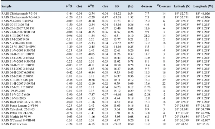
The gypsum deposited during the droughts of the Terminal Classic and early 102
Postclassic Periods was used to calculate the δ18O, δ17O and δD of the paleo-lake 103
water, which ranged from 3.6‰ to 4.9‰ for δ18O, 1.9‰ to 2.5‰ for δ17O, and 104
13.7‰ to 18.8‰ for δD (Fig. 1). Mean values of the paleo-lake waters (δ18O = 4.2‰; 105
δ17O = 2.2‰; δD = 16.4‰) during drought episodes are enriched in the heavier 106
isotopes compared to modern lake values (δ18O = 3.1‰; δ17O = 1.6 ‰; δD = 12.7‰). 107
5 was calculated using Bayesian age-depth analysis of radiocarbon ages obtained from 109
the sediment cores (3) (Fig. 1). The probabilities of drought occurring specifically 110
during the onset (~750 to ~850 C.E) and the end (~950 to ~1050 C.E.) of the TCP are 111
high (P > 0.85 and P > 0.95, respectively) (20). Multiple proxy climate records across 112
the Maya Lowlands also provide evidence of drought synchronicity, with only slight 113
temporal variations across the region (10). 114
115
To estimate quantitatively the magnitude of drought during the TCP, we 116
employed a transient model that explicitly simulates the evolution of the isotopic and 117
chemical composition of the lake water, including the gypsum flux to the lake 118
sediments (Fig. S3). The modeled gypsum flux can be compared to observed 119
variations in the gypsum content of the sediments, as expressed by variations in 120
sediment bulk density (3). Changes in lake surface-area-to-volume ratio were 121
obtained from the lake bathymetry (Fig. S4). The model was run at sub-monthly 122
resolution in a series of millennial-duration experiments, forced with North American 123
Regional Reanalysis (NARR) data for local precipitation and RHn. We first tested the
124
model using the climate forcing across the modern sampling period from 1994 to 125
2010 (Fig. S5). It successfully reproduced the mean of modern isotope data, with 126
insignificant gypsum precipitation. This time interval, which was fortuitously one of 127
the driest of recent decades, was then used as the baseline for comparison to paleo-128
simulations. 129
130
To provide scenarios that are directly comparable to the GHW data, we 131
performed long transient simulations in which rainfall and RHn were reduced by
132
variable amounts to simulate a series of multi-decadal-scale droughts. The use of a 133
model allows us to compare, directly and quantitatively, climate conditions that affect 134
the modern lake, with those of plausible drought conditions. First, only the intervals 135
over which the model produced gypsum deposition (modeled sediment density >1.1 136
g/cm3) were selected. The periods of modeled gypsum accumulation were then 137
aggregated into drought conditions for a given scenario via two pathways: (i) all 138
model variables were averaged across all of the droughts, and (ii) probability density 139
6 decadal-length drought. Data consistent scenarios were then selected by excluding 141
those model runs that fell outside the 1σ range of the isotope data and where, on 142
average, the model failed to produce significant gypsum accumulation (cutoff of 143
average density <1.2 g/cm3 based on 1σ range; Fig. S6). Two possible scenarios were 144
tested subsequently: (i) a reduction in precipitation with accompanying shifts in the 145
isotopic composition of rainwater (i.e. the amount effect) and, (ii) a reduction in 146
precipitation with accompanying decreases in RHn (Fig. 3).
147 148
In the first scenario, precipitation δ18O was reduced with an increase in rainfall 149
according to the amount effect relationship (i.e., δ18Oprecipitation/ΔPrecipitationvolume = –
150
0.0121‰/mm; Fig. S7) with associated changes in δD and δ17O that track the Global 151
MWL (i.e., no changes in d-excess or 17O-excess). No scenarios with these 152
assumptions are able to reproduce the relationship between δ18O, d-excess and 17 O-153
excess observed in the data. If the constraints provided by d-excess and 17O-excess 154
are removed and only δ18O and gypsum precipitation are employed, our model 155
permits reductions in precipitation that average 50% over all drought intervals (Fig. 3, 156
blue lines). This estimate is in broad agreement with previous work that relied on 157
carbonate δ18O-derived precipitation estimates (using the local amount effect), which 158
predicted reductions of up to 40% (6, 13). Our greater estimate of 50% is in part a 159
consequence of the peak drought δ18O values recorded by gypsum, as well as the 160
integration of simulated gypsum formation and true lake bathymetry in the model. 161
Crucially, however, the added information from the d-excess and 17O-excess data
162
suggests that multi-decadal shifts in the δ18O of precipitation (caused by the amount
163
effect) were not the dominant factor that affected the isotope budget of Lake 164
Chichancanab during the TCP. 165
166
In the second scenario, we reduced precipitation without changes in the δ18O 167
of precipitation, but instead with concurrent changes in RHn. In this case we observed
168
excellent agreement between the modeled evolution of all isotopic data, with 169
increases in δ18O accompanied by decreases in d-excess and 17O-excess (Fig. 3, red 170
lines). This analysis yielded plausible scenarios of precipitation reduction that average 171
47% across all droughts (with a 1σ level of 41-54%) accompanied by RHn reductions
7 of 4% (1σ level 2-7%). This result provides a robust, quantitative estimate of the 173
mean annual hydrological conditions of the combined drought periods during the TCP 174
at Lake Chichancanab. 175
176
Although the time evolution of our model is not a direct reconstruction of 177
climate conditions, the model permits heterogeneity within and between each decade-178
long drought. The ±1σ range determined from the probability density functions 179
indicates that the precipitation reduction could vary from 20 to 70% throughout the 180
modeled droughts (Fig. 3). This variability represents the transition into and out of 181
drought phases and demonstrates that the severity of the droughts could be intense (up 182
to a 70% reduction in precipitation), while maintaining the isotope balance and 183
without desiccating the lake. Although variability in the seasonal delivery of rainfall 184
(or lack thereof) is difficult to constrain because the residence time of the lake water 185
is greater than an annual cycle, our results provide quantitative estimates for the total 186
annual reduction in the water available for agriculture and domestic use for the 187
ancient Maya. Importantly, recorded Colonial-period accounts of later droughts, e.g., 188
1535-1560 and 1765-1773, during which high mortality, famines, and population 189
displacement were reported (30), are not manifest as intervals of gypsum precipitation 190
in Lake Chichancanab. The lack of gypsum formation is likely a result of shorter 191
duration and/or lower severity of these droughts, providing further evidence that the 192
TCP was an unusually dry period for the Holocene on the Yucatán Peninsula. 193
194
Using triple oxygen and hydrogen isotope data to independently deconvolve 195
climate variables precipitation, RHn and the amount effect, we constrained the
196
changing hydrological conditions at Lake Chichancanab. This approach provides a 197
significant advance over previous attempts to estimate the magnitude of rainfall 198
reduction during the TCP droughts (e.g. 6, 13). Furthermore, these quantitative 199
estimates of past rainfall and RHn can serve as input variables in crop models, to
200
better understand how drought affected agriculture (e.g., maize production) in the 201
8
References:
203 204
[1] D. A. Hodell, J. H. Curtis, M. Brenner. Possible role of climate in the collapse of 205
Classic Maya civilization. Nature375 (6530), 391-394 (1995). 206
207
[2] D. A. Hodell, M. Brenner, J. H. Curtis, T. Guilderson. Solar forcing of drought 208
frequency in the Maya lowlands. Science292 (5520), 1367-1370 (2001). 209
210
[3] D. A. Hodell, M. Brenner, J. H. Curtis. Terminal Classic drought in the northern 211
Maya lowlands inferred from multiple sediment cores in Lake Chichancanab 212
(Mexico). Quat. Sci. Rev. 24 (12), 1413-1427 (2005). 213
214
[4] J. H Curtis, D. A. Hodell, M. Brenner. Climate variability on the Yucatán 215
Peninsula (Mexico) during the past 3500 years, and implications for Maya cultural 216
evolution. Quat. Res. 46 (1), 37–47 (1996). 217
218
[5] G. H. Haug, D. Günther, L. C. Peterson, D. M. Sigman, K. A. Hughen, B. 219
Aeschlimann. Climate and the collapse of Maya civilization. Science 299, 1731–35 220
(2003). 221
222
[6] M. Medina-Elizalde S. J. Burns, D. W. Lea, Y. Asmerom, L. von Gunten, V. 223
Polyak, M. Vuille, A. Karmalkar. High resolution stalagmite climate record from the 224
Yucatán Peninsula spanning the Maya Terminal Classic period. Earth Planet. Sci.
225
Lett. 298 (1), 255-262 (2010).
226 227
[7] D. J. Kennett, S. F. Breitenbach, V. V. Aquino, Y. Asmerom, J. Awe, J. U. 228
Baldini, P. Bartlein, B. J. Culleton, C. Ebert, C. Jazwa, M. J. Macri. Development and 229
disintegration of Maya political systems in response to climate change. Science 338, 230
788–791 (2012). 231
9 [8] D. Wahl, F. Estrada-Belli, L. A. Anderson. 3,400 year paleolimnological record of 233
prehispanic human–environment interactions in the Holmul region of the southern 234
Maya lowlands. Palaeogeogr. Palaeoclimatol. Palaeoecol. 379–380, 17–31 (2013). 235
236
[9] P. M. Douglas, M. Pagani, M. A. Canuto, M. Brenner, D. A. Hodell, T. I Eglinton, 237
J. H. Curtis. Drought, agricultural adaptation, and sociopolitical collapse in the Maya 238
lowlands. Proc. Natl. Acad. Sci. 112 (18), 5607-5612 (2015). 239
240
[10] P. M. Douglas, A. A. Demarest, M. Brenner, M. A. Canuto. Impacts of climate 241
change on the collapse of lowland Maya civilization. Annu. Rev. Earth Planet. Sci.
242
44, 613-645 (2016). 243
244
[11] P. M. Douglas, M. Brenner, J. H. Curtis. Methods and future directions for 245
paleoclimatology in the Maya lowlands. Glob. Planet. Change138, 3-24 (2016). 246
247
[12] J. Yaeger, D. A. Hodell. Climate-culture-environment interactions and the
248
collapse of Classic Maya civilization. In: D. H. Sandweiss and J. Quilter (Eds.), El
249
Nino, Catastrophism, and Culture Change in Ancient America, Dumbarton Oaks, pp.
250
187-242 (2008). 251
252
[13] M. Medina-Elizalde, E. J. Rohling. Collapse of Classic Maya civilization related 253
to modest reduction in precipitation. Science335 (6071), 956-959 (2012). 254
255
[14] F. Gázquez, M. Morellón, T. K. Bauska, D. Herwartz, J. Surma, A. Moreno, M. 256
Staubwasser, B. Valero-Garcés, A. Delgado-Huertas, D. A. Hodell. Triple oxygen and 257
hydrogen isotopes of gypsum hydration water for quantitative paleo-humidity 258
reconstruction. Earth Planet. Sci. Letts.481, 177-188 (2018). 259
260
[15] H. Craig, L. I. Gordon. Deuterium and oxygen 18 variations in the ocean and the 261
marine atmosphere. Pp. 9–130. In E. Tongiorgi (ed.),.Stable isotopes in
262
oceanographic studies and paleotemperatures. Consiglio nazionale delle ricerche,
263
10 265
[16] J. R. Gat. Oxygen and hydrogen isotopes in the hydrologic cycle. Annu. Rev.
266
Earth Planet. Sci. 24, 225–262 (1996).
267 268
[17] D. Herwartz, J. Surma, C. Voigt, S. Assonov, M. Staubwasser. Triple oxygen 269
isotope systematics of structurally bonded water in gypsum. Geochim. Cosmochim.
270
Acta209, 254–266 (2017). 271
272
[18] B. Luz, E. Barkan. Variations of 17O/16O and 18O/16O in meteoric waters. 273
Geochim. Cosmochim. Acta74, 6276–6286 (2010).
274 275
[19] J. Surma, S. Assonov, M. J. Bolourchi, M. Staubwasser. Triple oxygen isotope 276
signatures in evaporated water bodies from the Sistan Oasis, Iran. Geophys. Res. Lett.
277
42, 8456–8462 (2015). 278
279
[20] Materials and methods are available as supporting material on Science Online. 280
281
[21] Z. Sofer. Isotopic composition of hydration water in gypsum. Geochim.
282
Cosmochim. Acta42, 1141–1149 (1978).
283 284
[22] D. A. Hodell, A. V. Turchyn, C. J. Wiseman, J. Escobar, J. H. Curtis, M. 285
Brenner, A. Gilli, A. D. Mueller, F. Anselmetti, D. Ariztegui, E. T. Brown. Late 286
Glacial temperature and precipitation changes in the lowland Neotropics by tandem 287
measurement of δ18O in biogenic carbonate and gypsum hydration water. Geochim.
288
Cosmochim. Acta77, 352–368 (2012).
289 290
[23] N. P. Evans, A. V. Turchyn, F. Gázquez, T. R. Bontognali, H. J. Chapman, D. A. 291
Hodell. Coupled measurements of δ18O and δD of hydration water and salinity of 292
fluid inclusions in gypsum from the Messinian Yesares member, Sorbas Basin (SE 293
Spain). Earth Planet. Sci. Lett.430, 499–510 (2015). 294
11 [24] F. Gázquez, N. P. Evans, D. A. Hodell. Precise and accurate isotope fractionation 296
factors (α17O, α18O and αD) for water and CaSO
4·2H2O (gypsum). Geochim.
297
Cosmochim. Acta198, 259–270 (2017).
298 299
[25] F. Gázquez, J. M. Calaforra, N. P. Evans, D. A. Hodell. Using stable isotopes 300
(δ17O, δ18O and δD) of gypsum hydration water to ascertain the role of water 301
condensation in the formation of subaerial gypsum speleothems. Chem. Geol. 452, 302
34-46 (2017). 303
304
[26] F. Gázquez, I. Mather, J. Rolfe, N. P. Evans, D. Herwartz, M. Staubwasser, D. A. 305
Hodell. Simultaneous analysis of 17O/16O, 18O/16O and 2H/1H of gypsum hydration 306
water by cavity ring-down laser spectroscopy. Rapid Commun. Mass Spectrom.
307
29(21), 1997-2006 (2015). 308
309
[27] T. Kluge, H. P. Affek. Quantifying kinetic fractionation in Bunker Cave 310
speleothems using Δ47. Quat. Sci. Rev.49, 82–94 (2012). 311
312
[28] M. S. Lachniet. Climatic and environmental controls on speleothem oxygen-313
isotope values. Quat. Sci. Rev.28(5), 412–432 (2009). 314
315
[29] L. I. Wassenaar, S. L. Van Wilgenburg, K. Larson, K. A. Hobson. A 316
groundwater isoscape (δD, δ18O) for Mexico. J. Geochem. Explor. 102, 123–136
317
(2009). 318
319
[30] J. A. Hoggarth, M. Restall, J. W. Wood, D. J. Kennett. Drought and its 320
demographic effects in the Maya lowlands. Current Anthropology, 58(1), 82–113 321
12
Figures:
323
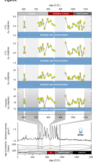
324
Fig. 1: Water isotopes during drought periods compared to modern water isotopes of 325
Lake Chichancanab. (Lower) Sediment density record of core CH1 7-III-04 from 0 326
to 2000 C.E. (shown relative to Maya chronology) (3). Periods of gypsum 327
precipitation are indicated by density values >1.1 g/cm3. Age uncertainty (95% 328
confidence intervals) are derived from Bayesian age-depth analysis and normalized to 329 S ed im en t d en si ty (g/cm 3)
CLASSIC TC POSTCLASSIC CONTACT
PRECLASSIC
MODERN LAKE WATER RANGE
POSTCLASSIC CLASSIC TERMINAL CLASSIC
Age (C.E.)
Age (C.E.)
Drier
MODERN LAKE WATER RANGE MODERN LAKE WATER RANGE MODERN LAKE WATER RANGE
A ge U nc er ta in ty (Y ears)
0 400 800 1200 1400 2000
1.0 1.5 -12 -16 -20 10 15 20 1.5 2.0 2.5 3.0 4.0 5.0
600 700 800 900 1000 1100
600 700 800 900 1000 1100
13 the best-fit age model (20) (Fig. S8). (Upper) δ18O, δ17O, δD and d-excess (δD – 8 ·
330
δ18O) of paleo-lake water data (yellow circles) from 550 to 1150 C.E shown after
331
correction of measured GHW for known fractionation factors (24) at 26°C. Horizontal 332
blue band defines the mean (±1σ) isotopic composition recorded in the modern lake. 333
Positive δ18O, δ17O and δD values and negative d-excess values reflect periods of 334
drought. Note d-excess axis is reversed. Abbreviation: VSMOW, Vienna Standard 335
14
337
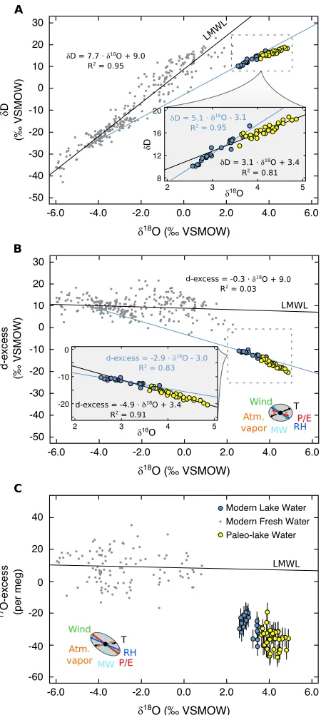
Fig. 2: Comparison of measured local meteoric water (gray circles), modern lake 338
water (blue circles) and paleo-lake water data (yellow circles). Paleo-lake water data 339
are shown after correction of measured GHW for known fractionation factors (24) at 340
26°C. In (A) δ18O vs δD, (B) δ18O vs d-excess (d-excess = δD – 8 · δ18O) and (C) 341
δ18O vs 17O-excess (17O-excess = ln[δ17O + 1] – 0.528 ln[δ18O + 1]) space, local 342
meteoric water measurements define the local meteoric water line (LMWL). Paleo-343
lake water in A, B and C displays greater enrichment along an evaporative trend 344
δ18O
LMW L
δD = 7.7 · δ18O + 9.0
R2 = 0.95
d-excess = -0.3 · δ18O + 9.0
R2 = 0.03
Modern Lake Water Modern Fresh Water Paleo-lake Water
LMWL 8
12 16
2 3 4 5
-20 -10 0
2 3 4 5
-6.0 -4.0 -2.0 0.0 2.0 4.0 6.0
-50 -40 -30 -20 -10 0 10 20 30
-6.0 -4.0 -2.0 0.0 2.0 4.0 6.0
-50 -40 -30 -20 -10 0 10 20 30
-6.0 -4.0 -2.0 0.0 2.0 4.0 6.0
-60 -40 -20 0 20 40 20
δD = 5.1 · δ18O - 3.1 R2 = 0.95
δD = 3.1 · δ18O + 3.4
R2 = 0.81
d-excess = -4.9 · δ18O + 3.4
R2= 0.91
d-excess = -2.9 · δ18O - 3.0 R2 = 0.83
P/E MW Wind Atm. vapor T RH P/E MW Wind Atm. vapor T RH LMWL δ D (‰ V S MO W ) 17 O -exces s (per meg) d-exces s (‰ V S MO W )
δ18O
δ
D
A
C B
δ18O (‰ VSMOW)
δ18O (‰ VSMOW)
[image:14.595.99.324.75.576.2]15 compared to modern lake waters. The grey ellipses define relative influence of 345
variables that can affect the isotopic composition of water in δ18O vs d-excess and
346
δ18O vs 17O-excess space; Precipitation/Evaporation (P/E), normalized relative
347
humidity (RHn), temperature (T), changes to source composition (MW), the degree of
348
equilibrium between atmospheric vapor and fresh water (Atm. vapor), and turbulence 349
created by wind (Wind)(14). The size of each arrow is derived from the tolerance 350
16 352
353
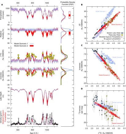
Fig. 3: (A) Transient model of the lake system from 550 to 1200 C.E. GHW data 354
(yellow circles) and core density are plotted against sampling ages derived from 355
Bayesian age-depth analysis (20). Multi-decadal-scale droughts were simulated by 356
forcing (1) a reduction in precipitation with accompanied shifts in the isotopic 357
composition of rainwater (i.e., the amount effect: δ18Oprecipitation/ΔPrecipitationvolume =
358
–0.0121‰/mm; Scenario 1, blue line) and (2) reductions in precipitation with 359
accompanied decreases in RHn (Scenario 2, red field). Probability density functions
360
incorporate the variability within and between each decade-long drought (GHW data 361
= yellow line; scenario 1 = blue line; scenario 2 = red line). Scenario 1 fails to match 362 x10-3 P reci pit at ion (m m /year) 1000 500 0 80 75 70 65 60
600 800 1000
A Relat iv e Hum idit y (%) δ 18O (‰ V S MO W ) 6 5 4 3 -10 -15 -20 -25 -30 d-ex cess (‰ V S MO W ) 15 14 13 12 11 Lake Dept h (m ) 2.0 1.8 1.6 1.4 1.2 1.0 Densit y (g/ cm 3) Model ed G ypsum P reci pit at ion
600 800 1000
Age (C.E.) δ18O (‰ VSMOW)
δ D (‰ V S M O W ) 20 18 16 14 12 10
2.0 2.5 3.0 3.5 4.0 4.5 5.0 5.5
Modern Lake Water Paleo-lake Water Modeled Gypsum Precipitation No gypsum precipitation
Model Scenario 1
Model Scenario 2
-10 -12 -14 -16 -18 -20 -22 -20 -30 -40 -50
2.0 2.5 3.0 3.5 4.0 4.5 5.0 5.5
2.0 2.5 3.0 3.5 4.0 4.5 5.0 5.5
d-ex cess (‰ V S M O W ) 17O -ex cess (per m eg)
Model Scenario 2
Model Scenario 1
Model Scenario 2 Model Scenario 1 B
C
D Probability Density
Function (PDF)
[image:16.595.93.504.92.529.2]17 the d-excess data derived from GHW. Scenario 2 successfully reproduces all δ18O and 363
d-excess data. When all model variables were averaged across all droughts, the mean 364
precipitation and RHn reduction (closed red boxes adjacent to PDFs) is 47% (with a
365
1σ level of 41-54%) and 4% (1σ level 2-7%), respectively. The ±1σ range determined 366
from probability density functions (open red boxes adjacent to PDFs) shows the 367
variability of precipitation and RHn throughout the droughts. Scenarios 1 and 2 are
368
also plotted as (B) δ18O vs δD, (C) δ18O vs d-excess and (D) δ18O vs 17O-excess. 369
Open circles indicate points in the model at which gypsum is precipitating; dots 370
indicate modeled data points when gypsum is not precipitating. Error bars (±1σ) are 371
18
Acknowledgments:
373
We thank James Rolfe for technical assistance and support with stable isotope 374
measurements, and three anonymous reviewers for insightful comments that 375
improved the paper. Funding: The research leading to these results received funding 376
from the European Research Council under the European Union’s Seventh 377
Framework Program (FP/2007-2013)/ERC grant agreement n. 339694 (Water 378
Isotopes of Hydrated Minerals) to D.A.H. Author Contributions: D.A.H., N.P.E. 379
and F.G. developed the analytical method and designed the study. M.B., J.H.C., and 380
D.A.H. collected the original sediment cores from Lake Chichancanab. N.P.E. 381
sampled the cores, and N.P.E. and F.G. performed all isotopic analyses. T.K.B. 382
designed the transient model and performed drought simulations. N.P.E., T.K.B. and 383
D.A.H. wrote the paper with contributions from all other authors. Competing
384
Interests: The authors declare no competing interests. Data Availability: All data are 385
available in the manuscript or supplementary material, and at 386
www.ncdc.noaa.gov/paleo/study/24476. 387
388
Supporting Online Material:
389
Materials and Methods 390
Modeling 391
Table S1 – S10 392
Fig S1 – S11 393
19 395
396 397 398
Supplementary Materials for
399 400
Quantification of Drought During the Collapse of the Classic Maya
401Civilization
402403
Nicholas P. Evans*, Thomas K. Bauska, Fernando Gázquez, Mark Brenner, Jason H. 404
Curtis, and David A. Hodell. 405
406
correspondence to: [email protected] 407
408 409
This PDF file includes:
410 411
Materials and Methods (Section 1.0) 412
Modeling (Section 2.0) 413
Tables S1 to S10 414
Figs. S1 to S11 415
20
1.0 Materials and Methods:
417 418
1.1 Sediment Cores and Sampling:
419 420
Lake Chichancanab is located at ~19°51’21”N 88°45’49”W, Yucatán 421
Peninsula, SE Mexico (Fig. S1). In March 2004, core CH1 7-III-04 was collected 422
from Lake Chichancanab with a piston corer in 14.7 m of water (3). Shortly after 423
collection, cores were split, wrapped in plastic film and stored at 4°C. Core sections 424
were measured for bulk density by gamma-ray attenuation by Hodell et al. (3), and 425
contain high-density gypsum bands interbedded with low-density organic layers (Fig. 426
S2). Gypsum was sampled at 0.5 cm intervals – individual crystals were picked from 427
the >350 µm size fraction and ground to a powder. Powdered samples were dried in 428
an oven at 45°C for 15-20 hours and placed under vacuum (~10-3 mbar) for ~3 hours 429
to remove adsorbed water prior to hydration water extraction (31). 430
431
1.2 Gypsum Hydration Water (GHW):
432 433
GHW was extracted from each sample (150-200 mg) by heating to 400°C and 434
trapping the evolved water, in vacuo, using a bespoke offline extraction system 435
described in Gázquez et al.(26). Triple oxygen (16O, 17O, 18O) and hydrogen (H, D) 436
isotopes of the GHW were measured by cavity ring down spectroscopy (CRDS) in the 437
Godwin Laboratory, University of Cambridge, UK (Table S1), using an L2140-i 438
Picarro CRDS water isotope analyzer with an attached micro-combustion module 439
(MCM; Picarro Inc.) (26, 32). The MCM’s cartridge was filled with a pyrolytic 440
catalyst to remove any organic contaminants in the GHW that may spectroscopically 441
interfere with the CRDS analyses (26). Triple oxygen and hydrogen isotope results 442
are reported in parts per thousand (‰) relative to V-SMOW. External error (1σ) was 443
estimated by repeated analysis (n = 11) of an analytical-grade standard extracted 444
along with the samples (26). Internal standards were calibrated previously against V-445
SMOW, GISP, and SLAP for δ18O and δD, and against V-SMOW and SLAP for 446
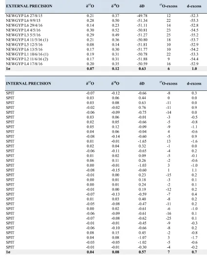
δ17O-δ18O (33). 1σ was ±0.07‰ for δ17O, ±0.12‰ for δ18O, ±0.63‰ for δD, ±0.8‰ 447
21 449
d-excess and 17O-excess are defined as:
450 451
d-excess = δD – 8 ·δ18O 452
17O-excess = ln (δ17O + 1) – 0.528 ln (δ18O + 1)
453 454
Where 0.528 is the slope of the modern δ17O - δ18O Global MWL(34). 455
456
Whereas study of GHW in lakes has produced relevant paleoclimatic records 457
that agree closely with other local and regional climate proxies (14, 22-24, 35, 36), 458
GHW can undergo post-depositional isotopic exchange under certain conditions (e.g. 459
temperature fluctuations >60°C during sediment burial and exhumation cycles) (37,
460
38). We suggest the gypsum in Lake Chichancanb preserves the isotopic composition 461
of the lake water at the time of deposition and has not undergone post-depositional 462
diagenesis or exchange with modern lake water. After applying fractionation factors, 463
the isotopic values of the paleo-lake waters are considerably enriched compared to the 464
modern lake (Fig. 1; Fig. S2). If the GHW had exchanged with sediment pore water, a 465
relatively homogeneous isotopic profile, with values similar to the current lake water, 466
would be expected. What is more, the burial depth of the gypsum is shallow (< 2 m) 467
and the sediments are porous, thus isotopic gradients in pore water would be strongly 468
attenuated by diffusion and advection with overlying lake water(14). 469
470
1.3 Precipitation, meteoric and lake water samples:
471 472
We report the triple oxygen and hydrogen isotopic measurement of lake water 473
(n = 156), river and ground water (n = 92), and rainwater (n = 31) samples from 474
stations across the Yucatán Peninsula, collected from 1994 to 2010 (Fig. S10; Tables 475
S3, S4 and S5). Measurements were made using an L2140-i Picarro CRDS water 476
isotope analyzer. The majority of rainwater samples were collected at 20°00'59"N 477
89°01'13"W, ~30 km west of Lake Chichancanab (22). All water samples were 478
collected and stored in Qorpak bottles with Polyseal cone-lined caps to prevent 479
22 481
1.4 Biogenic carbonate measurements:
482 483
Shells and shell fragments of the gastropod Pyrgophorus coronatus were 484
picked from 0.5 cm intervals of core CHI 7-III-04. Shells were cracked and sonicated 485
in methanol to remove contaminant debris. Subsequently, samples were treated with 486
10% H2O2 for 30 minutes to remove organic matter, dried and ground to a fine
487
powder. Stable oxygen isotopes of carbonate were measured using a ThermoScientific 488
GasBench II, equipped with a CTC autosampler coupled to a MAT253 mass 489
spectrometer(39). Samples were flushed with CP grade helium then acidified with 490
104% H3PO4 and reacted at 70°C for 1 hour. Repeat analysis of the Carrara Marble
491
standard yielded a 1σ analytical precision of ±0.1‰ for δ18O. Results are reported 492
relative to the Vienna Pee Dee Belemnite (VPDB). Small sample fragments were run 493
on a Kiel III carbonate preparation device interfaced with a Finnigan MAT 252 mass 494
spectrometer. Analytical precision was estimated at ±0.08‰ for δ18O. 495
496
1.5 Code:
497 498
All code can be found in the supplementary file 499
“Evans_et_al_2018_Matlab_Model” on Science Online. Please address enquiries to 500
T.K.B. ([email protected]). 501
502
2.0 Modeling:
503 504
2.1.1 Transient Model Details:
505 506
The transient box model presented here is a lake basin with a surface and deep 507
box (Fig. S4A). The volume (4.57e7 m3), surface area (1.02e7 m2), and surface area 508
to depth relationship conform to data presented in Hodell et al. (3) (Fig. S4B). This 509
geometry equates to a mean depth of 4.5 m in the model with the modern deepest area 510
of the basin equal to ~15 m. 511
23 The basin is fed by a precipitation flux determined by NARR reanalysis data 513
(~1 m water equivalent/m2/a; Fig. S5) with a constant catchment size through time.
514
The basin hydrology is effectively closed(40). Groundwater flux to and from the lake 515
(equivalent to ~10% of precipitation) delivers Ca2+, SO4-, Na2+, K+, Mg2+ and Cl- and
516
maintains the lake near the modern salt balance, with gypsum near saturation. Water 517
is lost via evaporation, which is held constant at a rate of 1.07 m water 518
equivalent/m2/a with the absolute flux evolving through time, depending on the 519
surface area of the lake. 520
521
The saturation state of gypsum was calculated offline with the PHREEQC 522
model for a wide range of solutions, starting at modern conditions. The lake model 523
incorporates these solutions in a look-up table to calculate the gypsum saturation at 524
every time step. If the lake exceeds saturation, Ca2+ and SO4- is removed by gypsum
525
precipitation at a rate that maintains the lake below saturation, with a response time of 526
1 year. Combining the mass of gypsum precipitated and surface area of the lake at a 527
given time-step allows us to calculate the gypsum accumulation in the lake sediment. 528
This is then used to calculate a synthetic core log of density, assuming the density of 529
accumulating gypsum is 2.31 g/cm3 and that the accumulation of other sediments is 530
constant at 0.941 mm/year, with a density of 1.06 g/cm3 based on the mean sediment 531
accumulation that brackets the drought periods. 532
533
2.1.2 Transient Model Isotope and Ionic Mass Balance:
534 535
The isotope mass balance model employs a Craig-Gordon evaporation scheme 536
(15) as formulated in Criss (41). The overall isotopic fractionation during evaporation 537
(αevp) depends on the equilibrium fractionation (αeq), kinetic fractionation (αkin),
538
relative humidity (h) and the isotopic ratio of water vapor (Rv) and the evaporating
539
surface of the basin (Rb), whereby:
540 541
𝛼"#$ = 𝛼"'𝛼()* 1 − ℎ
1 − 𝛼"'ℎR/
R0
(1)
24 543
Equilibrium fractionation (αeq) for H2O18 (α18Oeq) and DHO (αDeq) are
544
calculated using an assumed lake surface temperature of 25°C and the equations of 545
Horita and Wesolowski (42). The equilibrium fractionation for H2O17 is then a
546
function α18Oeq, where:
547 548
𝛼34O
"' = 𝛼36O"'7"'
549 550
and θeq is 0.529(43).
551 552
Kinetic fractionation factors for all three minor isotopes are calculated as a 553
function of wind-induced turbulence (w), lake surface temperature (T) and the kinetic 554
fractionation parameter between 18O and 17O (θkin):
555 556
𝛼36O
()* = 1.0283=
557
𝛼D()* = 1.25 − 0.02𝑇 𝛼36O
()*− 1 + 1
558
𝛼34O
()* = 𝛼36O()*7()*
559 560
We assume Rv depends on the degree to which the atmospheric water vapor
561
(veq) is in equilibriumwith Rp (44) where:
562 563
R/ = RB(αDE(BF/)V"')
564 565
The general form of the mass-balance equation for the mass of a given species (mX) 566
of either isotope or ion in basin box 1 (b1) is: 567
568
𝑑mX03
𝑑𝑡 = FMRM− FD/BRD/B+ FN03RN− F03NR03+ F0O03R0O− F030OR03
569
570
Similarly the mass balance for basin box 2 (b2) is: 571
25
𝑑mX0O
𝑑𝑡 = F030OR03− F0O03R0O
573
574
In this set of equations F represents the various fluxes of water in terms of mass of the 575
major water isotope (HHO16) and R represents the ratio of minor isotope or ionic 576
species relative to HHO16. As examples, the ratio of deuterium in box 1 is: 577
578
RPQR,03 = mDHO03
mHHO3U
03
579
580
The concentration of Ca in box 1 is: 581
582
R[WX],03 = mCa03
mHHO3U
03
583
584
When the overall water mass balance is calculated (i.e. the variation in volume): 585
586
RQQR\],03 = 1
587 588
Ratios for external isotopic such as the precipitation and groundwater fluxes are 589
referenced relative to VSMOW such that: 590
591
RPQR,B = δDB
10_ + 1 RPQR,`abRc
592
593
The isotopic ratios of the evaporation flux (Revp) are determined from Equation 1 and
594
the isotopic ratios of the basin surface (Rb1):
595 596
RD/B = R03
αD/B
597
26
2.1.3 Transient Model Parameterization:
599 600
When modeling the isotopic composition of the paleo-lake, the (1) lake 601
surface temperature (T), (2) wind-induced turbulence (w), (3) isotopic composition of 602
the atmospheric vapor, (4) salinity effect on isotope fractionation, and (5) the isotopic 603
composition of the freshwater input (and any variability caused by the amount effect) 604
must be known or assumed (Table S6). 605
606
1. To constrain water temperature changes at Lake Chichancanab during the 607
Terminal Classic Period (TCP), tandem measurements of both gypsum 608
hydration water (GHW) and carbonate δ18O that were deposited concurrently 609
permit the deconvolution of the δ18O carbonate signal into its temperature and 610
δ18O-water components via the carbonate paleo-temperature equation(22). To 611
calculate the temperature at which the aragonitic shells of Pyrgophorus
612
coronatus formed, we used the equation of Grossman and Ku (45) that is
613
based on analysis of foraminifera (Hoeglundina elegans) and gastropods: 614
615
T °C = 21.8 – 4.59(δ18Oarag PDB – δ18OwaterSMOW)
616 617
The δ18O of gastropod aragonite and GHW is used to estimate δ18Oarag and
618
δ18Owater, respectively. Gypsum and gastropod samples were only used if they
619
were in direct contact with each other, or the shell fragments were found 620
embedded within gypsum. The derived temperature from Pyrgophorus
621
coronatus and gypsum from the same bed averaged 25.9±1.7°C (Table S7).
622
This temperature is indistinguishable from the mean annual temperature of the 623
lake today (22). Equally, because 17O-excess is minimally affected by 624
temperature changes, moderate variations in mean temperature result in 625
insignificant effects on the trajectories of the evaporated waters. For example, 626
5°C of temperature change has a small effect on the model results for 17 O-627
excess (up to ∼±2 per meg in a terminal lake), whereas d-excess changes by as 628
much as ∼3‰ in a terminal lake, when all other parameters remain constant 629
27 631
2. It is known that the proportion of α18O
kin may be suppressed by turbulent flow
632
induced by wind(46), and therefore wind could alter isotope mass balance, 633
especially for d-excess and 17O-excess. The exponent ‘w’ is set between 0.5 634
(pure turbulence) and 1 (no wind). Measured wind speeds in the region of 635
Lake Chichancanab are ~3 m/s and relatively constant over the year (47), 636
resulting in a well-mixed lake-surface layer. When turbulence is not 637
considered, the model yields d-excess and 17O-excess values that are 638
systematically too low compared to the analytical data for some modern 639
periods. We also tested this variable by analyzing modern and paleo-lake 640
water data using previously published Monte Carlo models (14) (Section 641
2.1.5). These tests provide the best fit to modeled data when w is kept constant 642
at ~0.5 when modeling both the modern and the TCP GHW data. 643
644
3. The isotopic composition of modern atmospheric vapor is not well constrained 645
in the Yucatán Peninsula, nor are there estimates available for how this 646
variable has changed in the past. Assuming equilibrium with local meteoric 647
water, the isotopic composition of atmospheric water vapor can be 648
approximated (14). Gibson et al. (44), however, suggested that the isotopic 649
composition of atmospheric vapor is often only in partial equilibrium with that 650
of local freshwater. We assumed a degree of equilibrium of 60%, a reasonable 651
estimate for most tropical and inter-tropical regions(44). Note that Gázquez et 652
al.(14) show that the triple oxygen and hydrogen system is relatively sensitive 653
to the isotopic composition of the vapor, especially for coastal lakes affected 654
by advection of marine vapor masses. In coastal lakes, the isotopic 655
composition of the modern atmospheric vapor is in equilibrium with seawater 656
rather than freshwater. This is probably not the case at Lake Chichancanab, 657
which is located ~140 km inland. 658
659
4. High concentrations of NaCl and other salts within a lake can cause the water 660
isotopic activity ratios to diverge from the corresponding concentration ratios, 661
28 ionic hydration shells (17, 48). This “salt effect” is different for hydrogen and 663
oxygen isotope fractionation, resulting in complications when interpreting the 664
relationship between δ18O and δD at salt concentrations >100,000 mg/L(17,
665
48). The total dissolved salt concentration in Lake Chichancanab today is 666
~4000 mg/L(3). Substantial oxygen and hydrogen isotope fractionation effects 667
caused by high salinity would not be expected at these low concentrations (41,
668
48). During periods of lake drawdown, the transient model displays elevated 669
salt concentrations, but concentrations that approach 100,000 mg/L are never 670
experienced in model runs. 671
672
5. The mean (±1σ) modern isotopic composition of regional groundwater is -4.0 673
± 1.7‰ for δ18O, -2.10 ± 0.9‰ for δ17O and -23.5 ± 12.8‰ for δD. We used 674
δ18O = -4.5‰ and δD = -26‰ (so that d-excess = 10‰) and set 17O-excess = 675
2.5 per meg to model present-day conditions. These variables were held 676
constant throughout the transient model runs, although they can be 677
systematically varied to reflect isotope effects such as the amount effect (see 678
below and Section 2.1.4). We tested the effect of non-systematic variability on 679
the isotopic composition of meteoric water (using bounds of ±0.5‰ for δ18O, 680
±5‰ for d-excess, and ±9.5 per meg for 17O-excess), using the steady state 681
Monte Carlo model of Gázquez et al. (14) to quantify derived uncertainty 682
(Section 2.1.5). 683
684
The amount effect (i.e. correlation between depletion of heavy isotopes in 685
rainfall with greater amount of rain) is thought to play a role in the Yucatán 686
Peninsula and thus the isotopic composition of meteoric water may vary over 687
the timescales modeled (6, 13). The amount effect and its perturbation in the 688
δ18O of precipitation (P) over a seasonal cycle was calculated from isotopic 689
composition of precipitation collected at 20°00'59"N 89°01'13"W (22), and 690
rainfall amounts from the proximal meteorological station at Dziuche, 691
19°54'00"N 88°48'40"W, from 2006 to 2009. The linear regression (δ18O = -692
0.0176(P) - 0.1204; R² = 0.92) is very similar to that found by Medina-693
29 0.0118(P) - 0.64; R² = 0.80). We compiled data from Veracruz between 1969 695
and 1985 (omitting years with poor data coverage) and the records from 696
Chichancanab between 2006 and 2009(22). The compiled linear regression for 697
δ18O (δ18O = -0.0121(P) - 0.41) displays a significant correlation (R² = 0.73), 698
whereas there was no significant amount effect displayed by d-excess or 17 O-699
excess (Fig. S7). 700
701
2.1.4 Deconvolution of climatic variables:
702 703
δ18O, 17O-excess and d-excess are affected to differing degrees by changes in 704
RHn, the ratio P/E, temperature, turbulence (e.g., wind) on the water surface during
705
evaporation, the isotopic composition of the atmospheric water vapor, changes to the 706
isotopic composition of the input source (14, 19, 41, 44). In δ18O-17O-excess and 707
δ18O-d-excess space, the predicted trends of waters undergoing evaporation (in partial 708
equilibrium with atmospheric vapor) show that 17O-excess and d-excess are largely 709
sensitive to RHn and the ratio P/E, moderately sensitive to the isotopic composition of
710
freshwater input, turbulence on the water surface during evaporation and to the 711
isotopic composition of the atmospheric water vapor, whereas their sensitivities to 712
temperature are relatively small, especially for 17O-excess (Fig. 2)(14). Because the 713
isotopic composition of the freshwater input, along with variance in the turbulence on 714
the water surface during evaporation, the isotopic composition of the atmospheric 715
water vapor, and temperature are relatively well constrained (Section 2.1.3; Table S6), 716
variability in RHn, P/E and changes in the isotopic composition of the freshwater
717
input (caused by the amount effect) can be deconvolved in model scenarios. 718
719
To provide semi-realistic scenarios that are directly comparable to the GHW 720
data, transient simulations were run in which NARR precipitation and RHn forcings
721
were reduced by variable amounts to simulate a series of multi-decadal-scale droughts 722
(Fig. 3; Fig. S3). Precipitation and/or RHn forcings are directly modulated by the
723
density record of core CH1-III-04(3); the maximum variability during a run was set 724
to the maximum density point over time, and precipitation and/or RHn were reduced
725
linearly across all months. Absolute reductions in P/E and RHn were referenced
30 relative to mean NARR data over the period from 1994 to 2010. In other words, a 727
50% reduction in precipitation and a 5% reduction in RHn would equate to 50% less
728
rainfall in each month (e.g. 200mm/mth to 100mm/mth), and a decrease in the 729
absolute RHn by 5 percentage units each month (e.g. RHn = 75% to RHn = 70%)
730
during a modeled time period compared to the 1994 to 2010 baseline. 731
732
During model runs, the intervals of modeled gypsum accumulation were first 733
selected from a pre-determined density range (modeled sediment density >1.1 g/cm3). 734
The periods of modeled gypsum accumulation were then aggregated into drought 735
conditions for a given scenario in two ways: (i) all model variables were averaged 736
across all the droughts, and (ii) probability density functions were constructed 737
incorporating the variability within and between each decadal-length drought (Fig. 738
S3). To identify the timing of significant gypsum accumulation, we selected periods 739
of modeled sediment density >1.2 g/cm3. This would be equivalent to selecting data 740
outside one standard deviation of the mean sediment density from core CH1-III-04 741
(1.09±0.11 g/cm3), calculated from the total sediment density record of Hodell et al.
742
(3) from 500 B.C. to 2000 C.E. (Fig. S6A). Modeled data from these periods were 743
then compared to mean (±1σ) GHW data. The model runs were selected as positive 744
when the modeled δ18O, d-excess and 17O-excess (during periods of significant 745
gypsum precipitation) fell within one standard deviation (1σ) of the GHW data (Fig. 746
S6). A major constraint on the modeled P/E variability is the sediment density range 747
from which the modeled data are selected. As displayed in Fig. S6, if the modeled 748
sediment density threshold is changed from 1.2 g/cm3, the lower bound of P/E and
749
RHn estimates will vary systematically. Importantly, increasingly conservative
750
estimates for periods of gypsum precipitation (i.e. modeled sediment density >1.2 751
g/cm3) produce increasingly more severe reductions in baseline P/E and RHn.
752 753
Two scenarios were tested: (i) a reduction in precipitation with accompanying 754
shifts in the isotopic composition of rainwater (i.e. the amount effect) and, (ii) a 755
reduction in precipitation with accompanying decreases in RHn. In scenario 1 (main
756
text; Fig. 3), the density record modulates changes in the P/E ratio. Modeled 757
31 relationship (i.e. δ18Oprecipitation/ΔPrecipitationvolume = –0.0121‰/mm; Fig. S7). As the
759
associated changes in δD and δ17O track the Global MWL, no changes in d-excess or
760
17O-excess are imposed in these scenarios. No scenarios were able reproduce the
761
relationship between δ18O, d-excess and 17O-excess observed in the data. In scenario 762
2, changes in the ratio P/E were coupled with changes to RHn.
763 764
It should also be noted that a combination of RHn reduction and the amount
765
effect could potentially reproduce the observed data during the TCP. Although a 766
combination of RHn reduction and (a suppressed) amount effect cannot be definitively
767
ruled out, given the great number of possible outcomes when modeling three variable 768
parameters, our experiments show that the amount effect does not dominate the 769
isotopic budget of the lake. Thus, any influence of the amount effect (in combination 770
with RHn reductions) at Lake Chichancanab during the TCP will have little effect on
771
modeled outcomes because of the dominance of RHn in the 17O-excess and d-excess
772
signal. 773
774
2.1.5 Monte CarloModeling Scenarios:
775 776
In addition to transient model experiments described above and in the main 777
body of the text, we also used a previously described steady state model of the lake in 778
a series of Monte Carlo experiments to determine the range of climatological 779
conditions that simultaneously satisfy all stable isotope results of GHW, in 780
combination with statistical estimates of uncertainty (Fig. S9) (14). In these scenarios, 781
the parameter “Xe” represents the hydrologic balance of the lake. A scenario in which 782
all water is lost by outflow and no evaporation occurs is represented as Xe = 0, 783
whereas a scenario in which all water is lost to evaporation (i.e. a terminal basin) is 784
represented as Xe = 1. The Xe of Lake Chichancanab is not believed to have changed 785
over the last ~1500 years and near-terminal conditions are thought to have prevailed 786
(40). Equally, Gázquez et al. (14) show that when Xe ranges from 0.75 to 1, changes 787
in this parameter barely affect the RHn values derived from this Monte Carlo model.
788
Here, we chose conservative estimates of Xe between 0.8 and 0.9 to cover all likely 789
32 791
Modeled GHW data suggest there was a reduction in RHn of between 2 and
792
9% during the TCP, compared to the period when modern lake water was sampled 793
(1994-2010), in good agreement with our transient experiments (2-7%) (Table S9). 794
Estimated errors for RHn are smaller than 4% (1σ) when all variables listed in Table
795
S8 are considered. The slightly greater estimates for reductions in RHn relative to the
796
transient model arise because the steady-state assumption in the Monte Carlo model 797
precludes an accurate simulation of isotopic balance during lake level fluctuations. 798
Because the model does not account for the additional isotopic enrichment in the lake 799
due to decreased P/E during a lake-level drawdown, it is slightly biased towards 800
higher estimates of RHn reduction.
801 802
2.2 Age Models:
803 804
Radiocarbon ages for core CH1 7-III-04 were obtained by Hodell et al. (3). 805
We estimated calendar ages with 95% confidence intervals using the Bayesian Age-806
Depth Modeling software “BACON” in R (Fig. S8) (49). Derived age-depth error 807
(95% confidence intervals) was normalized to the best-fit line to produce age-depth 808
errors for the Chichancanab density record (3) (Fig. 1; Table S10). To quantify age 809
uncertainty in relation to the timing of dry intervals, we inverted the density record of 810
core CH1-III-04 and identified data outside one standard deviation of the mean 811
sediment density from core CH1-III-04. This would be equivalent to selecting 812
sediment densities >1.2 g/cm3, equivalent to the periods from which GHW was
813
extracted. The BACON function ‘Events’ was then used to quantify the probability of 814
arid conditions at any calendar age. Fifty-year window widths were used, with the 815
windows moving at 10-year steps from the core's bottom ages to its top (Fig. S11) 816
(49). 817
818
We also used Bayesian age modeling techniques to synthesize the regional 819
proxy records of Curtis et al. (4), Wahl et al. (8) and Douglas et al. (50) (Fig. S11). To 820
quantify age uncertainty in relation to the timing of dry intervals, we inverted the 821
33 and Douglas et al. (50), and the 5-point smooth of the δ18O Cytheridella ilosvayi
823
record from Curtis et al. (4). 824
825
All proxy records dated using radiometric techniques yielded a significant age 826
uncertainty. Overall, although individual records show subtle variations in drought 827
timing, the age uncertainty results in the chance of drought occurring any time 828
between 500 and 1300 C.E.(51). Gypsum deposition at Lake Chichancanab displays a 829
significant chance of occurring from ~750 to ~850 C.E (Probability of drought at 800 830
C.E. = 0.85), coinciding with the onset of the collapse of Terminal Classic Maya 831
34
Supplementary Tables:
[image:34.595.91.500.256.597.2]833 834
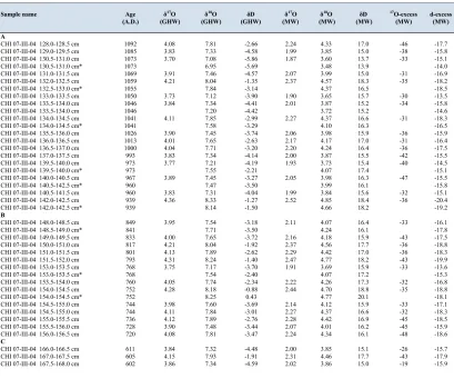
Table S1:
835
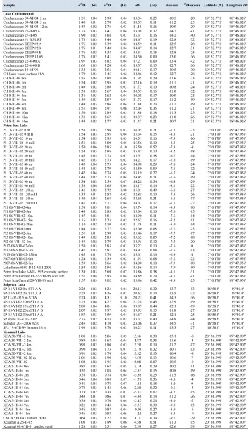
Isotopic composition of measured gypsum hydration water (GHW) and calculated 836
lake mother water (MW) from samples recovered from core CH1 7-III-04, Lake 837
Chichancanab. Asterisk denotes samples that were analyzed with the MCM of the 838
L2140-i Picarro CRDS turned off; δ17O results were considered unreliable(26)and 839
samples were not used in modeling analysis. 840
841
35
Table S2:
843
External and internal reproducibility of GHW measurements. 844
36
Table S3:
846
37
Table S3 Continued:
848
38
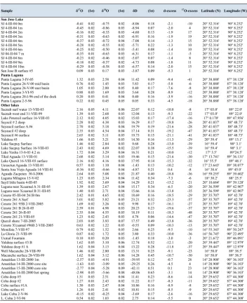
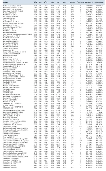
Table S4: Stable isotope ratios of river and freshwaters from the Yucatán Peninsula. 850
39
Table S5:
852
Stable isotope ratios of rainwater from the Yucatán Peninsula. 853
40
Table S6:
855
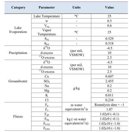
Transient model parameters. See text for details of parameters. 856
857
Category Parameter Units Value
Lake Evaporation
Lake Temperature °C 25
w - 0.5
Veq - 0.6
Vapor
Temperature °C 25
θeq - 0.529
θkin - 0.518
Precipitation
δ18O
(per mil, VSMOW)
-4.5
d-excess 10
17O-excess 2.5
Groundwater
δ18O
(per mil, VSMOW)
-4.5
d-excess 10
17O-excess 2.5
Ca
g/kg
0.607
SO4 2.455
Na 0.2
Mg 0.2
K 0.011
Cl 0.234
Fluxes
Fp m water
equivalent/m2/a
Reanalysis data = ~1
Fe 1.07
Fgb
kg (~m water equivalent/m2/a)
1.02e9 (~0.1)
Fbg 1.02e9 (~0.1)
Fb1b2 1.02e10 (~1.0)
Fb2b1 1.02e10 (~1.0)
[image:40.595.74.508.129.574.2]41
Table S7:
859
Paleo-lake temperature calculations. The equation of Grossman and Ku(45) was used 860
to calculate the temperature at which the aragonitic shells of Pyrgophorus coronatus
861
formed. 862
42
Table S8:
864
Steady-state parameters for Monte Carlo simulations. See text for details of 865
parameters. 866
867
Category Parameter Units Values [Range]
Lake Evaporation
Lake
Temperature °C [22 28]
w - [0.5 0.6]
Veq - [0.6 0.7]
Xe - [0.8 0.9]
Vapour
Temperature °C 25
θeq - 0.529
θkin - 0.518
Precipitation
δ18O
(per mil, VSMOW)
[-5 -4]
d-excess [5 15]
17Oexcess [-7 12]
43
Table S9:
869
Monte Carlo modeling solutions.n defines number of successful simulations. 870
44
Table S10:
872
Output table of Bayesian age-depth analysis. Mean ages display single ‘best’ model 873
based on the weighted mean age for each depth. Positive and negative age errors 874
45
Table S10 Continued:
876
46
Table S10 Continued:
878
47
Supplementary Figures:
880 881
882
Fig. S1: Map of the Maya Lowlands displaying the locations of proxy climate 883
archives (north to south); the Chaac speleothem of Tzabnah Cave(6); Punta Laguna 884
(4); Aguada X’caamal(52); Lake Chichancanab (this study)(1-3); Lake Puerto Arturo 885
(53); Laguna Yaloch(8); Macal Chasm(54); Lake Salpetén(9); the Yok I speleothem 886
of Yok Balum Cave(7). 887
100
0 200
km
21°N
20°N
19°N
18°N
17°N
16°N
84°W 85°W 86°W 87°W 88°W 89°W 90°W 91°W 92°W 93°W 94°W 95°W 96°W 97°W
A A
C B
B
C
D E
F
A B C
A B C
Caves: Lakes:
Punta Laguna Aguada X’caamal Lake Chichancanab Lake Salpetén Lake Puerto Arturo Laguna Yaloch Tzabnah Cave
Macal Chasm Yok Balum Cave
[image:47.595.126.476.132.388.2]