Psychophysical studies of interactions between luminance and chromatic information in human vision

(1)

PSYCHOPHYSICAL STUDIES OF INTERACTIONS

BETWEEN LUMINANCE AND CHROMATIC INFORMATION

IN HUMAN VISION

Stéphane Clery

A Thesis Submitted for the Degree of PhD

at the

University of St Andrews

2014

Full metadata for this thesis is available in

St Andrews Research Repository

at:

http://research-repository.st-andrews.ac.uk/

Please use this identifier to cite or link to this thesis:

http://hdl.handle.net/10023/6376

This item is protected by original copyright

(2)

Psychophysical studies of interactions

between luminance and chromatic information

in human vision

St´

ephane Clery

This thesis is submitted to the University of St Andrews

for the degree of PhD

(3)

(4)

1. Candidate’s declarations:

I, Stéphane Clery, hereby certify that this thesis, which is approximately 75 000 words in length, has been written by me, that it is the record of work carried out by me and that it has not been submitted in any previous application for a higher degree.

I was admitted as a research student in September 2009 and as a candidate for the degree of Doctor of Philosophy in September 2009; the higher study for which this is a record was carried out in the University of St Andrews between 2009 and 2013.

Date 25/10/2013 signature of candidate ______________

2. Supervisor’s declaration:

I hereby certify that the candidate has fulfilled the conditions of the Resolution and Regulations appropriate for the degree of Doctor of Philosophy in the University of St Andrews and that the candidate is qualified to submit this thesis in application for that degree.

Date 25/10/2013 signature of supervisor ______________

3. Permission for electronic publication: (to be signed by both candidate and supervisor)

In submitting this thesis to the University of St Andrews I understand that I am giving permission for it to be made available for use in accordance with the regulations of the University Library for the time being in force, subject to any copyright vested in the work not being affected thereby. I also understand that the title and the abstract will be published, and that a copy of the work may be made and supplied to any bona fide library or research worker, that my thesis will be

electronically accessible for personal or research use unless exempt by award of an embargo as requested below, and that the library has the right to migrate my thesis into new electronic forms as required to ensure continued access to the thesis. I have obtained any third-party copyright permissions that may be required in order to allow such access and migration, or have requested the appropriate embargo below.

The following is an agreed request by candidate and supervisor regarding the electronic publication of this thesis:

(iii) Embargo on both all of printed copy and electronic copy for the same fixed period of two years on the following ground(s):

publication would preclude future publication.

Date 25/10/2013 signature of candidate ____________ signature of supervisor ____________

(5)

(6)

Abstract

In this thesis, I investigated how human vision processes colour and luminance

infor-mation to enable perception of our environment. I first tested how colour can alter

the perception of depth from shading. A luminance variation can be interpreted as

either variation of reflectance (patterning) or variation of shape. The process of

shape-from-shading interprets luminance variation as changes in the shape of the object (e.g.

the shading on an object might elicit the perception of curvature). The addition of

colour variation is known to modify this shape-from-shading processing. In the

ex-periments presented here I tested how luminance driven percepts can be modified by

colour. My first series of experiments confirmed that depth is modulated by colour. I

explored a larger number of participants than previously tested. Contrary to previous

studies, a wide repertoire of behaviour was found; participants experienced variously

more depth, or less depth, or no difference. I hypothesised that the colour modulation

effect might be due to a low-level contrast modulation of luminance by colour, rather

than a higher-level depth effect. In a second series of experiments, I therefore tested

how the perceived contrast of a luminance target can be affected by the presence of

an orthogonal mask. I found that colour had a range of effects on the perception of

luminance, again dependant on the participants. Luminance also had a similar wide

range of effects on the perceived contrast of luminance targets. This showed that, at

supra-threshold levels, a luminance targets contrast can be modulated by a

compo-nent of another orientation (colour or luminance defined). The effects of luminance

and colour were not following a particular rule. In a third series of experiments, I

explored this interaction at detection levels of contrast. I showed cross-interaction

(7)

(8)

Acknowledgements

(9)

(10)

List of Figures

2.1 Absorbance spectra of cones and rods in humans . . . 4

2.2 Ganglion cell receptive field. . . 9

2.3 Description of the Naka-Rushton equation. . . 19

3.1 Spatial processing stages from original scene to processing by cones and post-receptoral channels. . . 24

3.2 Illustration of differential processing of luminance and chromatic channels. . 26

3.3 CSF function of luminance and chromatic channels . . . 26

3.4 Multiple channel hypothesis: Sets of luminance channels . . . 28

3.5 Temporal frequency tuning of luminance and chromatic channels . . . 29

3.6 Masking paradigm . . . 32

3.7 Example mask/target stimuli . . . 68

3.8 Example of mask/target configurations in masking experiments . . . 69

3.9 Dipper shape function . . . 70

3.10 Compressive contrast . . . 71

3.11 Adaptation effect and spatial structure . . . 72

3.12 Gilchrist lightness illusion . . . 73

4.1 Illuminant D65 and blackbody radiation at 6500 K . . . 76

4.2 Luminous efficiency functions . . . 78

4.3 Chromaticity functions . . . 80

4.4 Colour-matching functions standards . . . 81

4.5 Cone absorption functions . . . 83

5.1 Illustration of shading and stereo stimuli . . . 93

5.2 Illustration of all the stimuli used in the experiment. . . 96

5.3 Description of cumulative Weibull function parameters . . . 98

5.4 Description of inverse cumulative Weibull function parameters . . . 99

5.5 Results from condition 1 . . . 101

5.8 Parameters analysis between sinusoid and square-wave for condition 1. . . . 109

5.9 Results of retest: condition 3 . . . 117

6.1 Experiment II, stimuli-set . . . 131

6.2 Data visualization: raw data . . . 132

6.3 Data visualization: transformation . . . 134

6.4 Visualization of all results from experiment 2 . . . 135

(18)

6.6 Luminance mask effect versus colour mask effects . . . 142

6.7 Luminance mask effect versus colour masks effects: density . . . 143

6.8 Colour and luminance masks analysis by target values. . . 146

6.9 Luminance mask effects versus colour mask effects (adjusted) . . . 148

6.10 Colour and luminance mask analysis by target values with extended dataset.150 6.11 Drift analysis luminance mask . . . 152

6.12 Drift analysis colour mask . . . 153

6.13 Comparison between depth matching and contrast matching experiments . 156 7.1 Temporal wavefrom . . . 172

7.2 Example of psychometric function fitting procedure . . . 176

7.3 TvC curve, luminance mask D1/M1 . . . 177

7.6 TvC curve, luminance mask D4 . . . 178

7.7 Slope parameter for luminance mask, participant D1. . . 179

7.11 TvC curve, colour mask D1/M1 . . . 181

7.14 TvC curve, colour mask D4 . . . 182

7.15 Slope parameter for colour mask, participant D1/M1. . . 183

7.18 Slope parameter for colour mask, participant D4. . . 183

8.1 Luminance ratio and gun’s chromaticity values . . . 191

8.2 Relationship between L and M cone contrast amplitude modulations . . . . 195

8.3 Description of the behaviour of cone ratio metrics . . . 201

8.4 Results of minimum motion experiment: sinusoid and square-wave . . . 206

8.5 Results of minimum flicker experiment (part1) . . . 213

8.6 Results of minimum flicker experiment (part2) . . . 214

(19)

(20)

List of Tables

2.1 Bipolar cell types . . . 8

4.1 Standard Units used in Radiometry and Photometry . . . 76

5.1 Analysis results of condition 1 . . . 102

5.2 Fit results for condition 1 . . . 103

6.1 IDs of participants tested in both the depth and the contrast matching experiments . . . 128

6.2 Details of conditions tested are presented in mask\target pairs, in contrast (%). . . 130

6.3 Table of correlation metrics . . . 146

6.4 Table of correlation metrics, full dataset . . . 149

7.1 Participants ID tested in both detection and contrast matching experiments 170 7.2 Masks conditions tested for each participants . . . 173

(21)

List of abbreviations

2 IFC: two-interval forced choice

CIE: Commission International de l´ ´Eclairage CRF: classical receptive field

CSF: contrast sensitivity function DOG: difference of Gaussian model H-K effect: Helmholtz–Kohlrausch effect ERG: Electroretinogram

LGN: lateral geniculate nucleus

M (cells/layers): Magnocellular (cells/layers) P (cells/layers): Parvocellular (cells/layers) K (cells/layers): Koniocellular (cells/layers) RF: receptive field

SF: spatial frequency SFS: shape-from-shading

TvC: threshold versus (mask) Contrast VS: visual system

(22)

Glossary

Visual channel:

A visual channel is a perceptual sub-organization of visual information. There are three main pathways of visual information (see Chapter 3). Their operational definition consists of a recombination of retinal signals (L, M and S) into three distinct signals M-L, (M+L)-S & L+M, perceptually equivalent to red-green, yellow-blue, and luminance perception. As such, these channels are also called post-receptoral mechanisms. See Chapter 4 for an extended definition of photometry and colorimetry essential for the characterization of luminance and chromatic channels.

Visual pathway:

(23)

Chapter 1

General introduction

The processing of visual information by the human visual system involves a dedicated part of the central nervous system from the retina through the lateral geniculate nucleus (LGN) to Visual area 1 (V1) and higher cortical areas. This visual processing involves physiological pathways carrying specific types of information whose properties can be traced back to the ganglion cells in the retina. There are 3 physiological pathways of information processing carrying visual input to the cortex. A more detailed and in depth introduction to the physiology of colour and luminance vision (in the context of spatial information) will be given in Chapter 2.

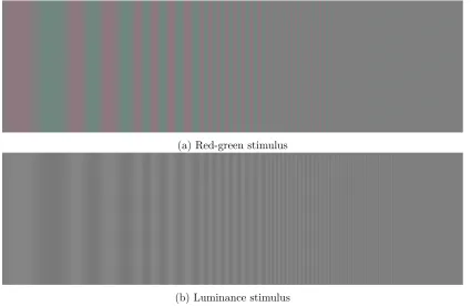
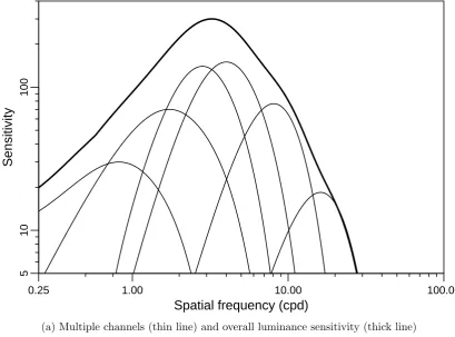
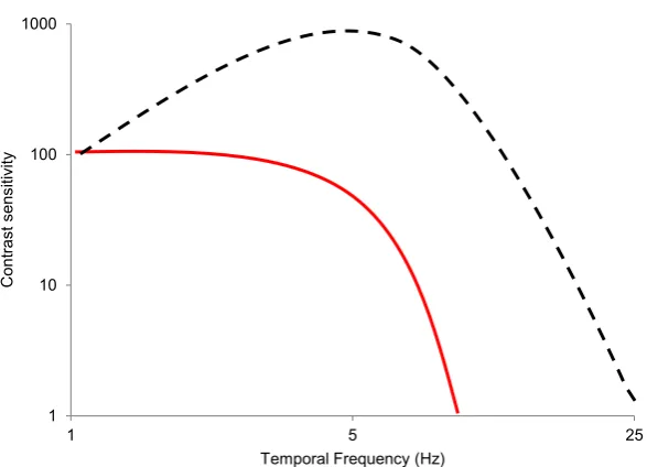
Before the physiological details of visual processing were known, psychophysical chan-nels of visual information had been suggested (e.g. M. D. Wright, 1946). A common suggestion is that three fundamental psychophysical channels exist; one channel carry-ing information about luminance and two about chromatic information. A psychophysical channel is defined operationally, through the use of psychophysical experiments. The stan-dardized psychophysical metrics used in this thesis will be reviewed in Chapter 4 (General Methods). It was found that luminance and chromatic channels had different properties in the way they respond to spatial and temporal information, for example they process visual information at different scales (e.g. Mullen, 1985). Channels can be said to be composed of orientation and spatial scale sub-channels. These concepts and data relating to them will be presented in the psychophysical review chapter (Chapter 3). A particular subject of interest is how these channels interact under differing conditions. This is studied because visual processing plays an important role for us to interpret and interact with our environment. One of the questions of this thesis is about the functional role of these chan-nels and interactions between them. In Chapters 2 and 3, I will review how orientation processing (part of the processing of edges) is achieved by interacting channels. In the experimental chapters, I will explore how luminance and colour interact in the processing of information at different levels. Furthermore, I will contrast results when possible with results from the processing of luminance-luminance interactions.

(24)

shape-from-shading (SFS) by isoluminant chromatic information. I will explore this phenomenon in a larger number of participants than previously tested. In the second experiment (Chap-ter 6), I will present data on how orthogonal components can modulate the perception of suprathreshold contrast. The effect of mask types (sinusoids with smooth edges or square-wave with straight edges) will be studied in a population of 12 participants. These orthogonal masks were defined both in luminance and in red-green isoluminant colours. The effects of target contrast, mask contrast and mask type (luminance or chromatic) will be detailed for 22 participants. In a third experiment (Chapter 7) the effects of orthogonal modulation upon the detection of a luminance target will be detailed. The masks could either be luminance or colour defined in this study.

(25)

Chapter 2

Physiology of luminance and

chromatic processing from the

retina to the cortex

2.1 Introduction

The aim of this introductory chapter is to present a short description of the physiological basis of information processing through separate pathways. This will be done with an emphasis on luminance and colour processing. In this chapter, I explore perception in terms of signal processing, starting from the retinae to the visual cortex, thereby focusing on the physiological mechanisms of perception. I will detail current knowledge of how luminance, chromatic, and spatial information are computed from the retina to the cortex. The following chapter, Chapter 3, follows the natural consequence of visual processing which is conscious perception, and is therefore oriented towards psychophysics. Chapter 3 will also focus on image/scene processing.

2.2 Retina

In cross-section, the retina is a layered structure, with the photoreceptor cells outer seg-ment at the most external layer. Other layers contain receptor bodies, horizontal cells, ganglion cells, and optic nerve fibres (for a more complete description see classic work by Polyak, 1941, 1957; Ramon y Cajal & Felipe, 1892). Visual processing starts when light1_{reaches the back of the eye, goes through the retinal layers to eventually be absorbed}

by photoreceptors; which then gets processed by intermediate cells followed by ganglions projecting to the cortex via the optic nerve.

I will first describe details of the cone photoreceptors, then the retinal processing done by intermediate and ganglion cells.

1

(26)

Wavelength

Absorbance (log unit)

350 400 450 500 550 600 650 700 750 800 850

−8

−7

−6

−5

−4

−3

−2

−1

0

1

[image:26.595.89.501.91.373.2]

L M S Rod

Figure 2.1: Absorbance spectra of cones and rods in humans, estimates by Stockman and Sharpe (2000, cones) and Kraft et al. (1993, rods).

2.2.1 Cones

Primates’ eyes have evolved two photoreceptors types: the cones and the rods. The cones are responsible for daylight viewing (photopic condition) and the rods are responsible for low-light vision (scotopic condition, see Chapter 4, General methods, for more details).

Humans and some other primates possess three types of cones, and are, therefore, referred to as trichromats. The three types of cones are called L, M, and S;2 for long, medium, and short absorption range (see Figure 2.1). Having multiple cone types means that at the initial processing step there are multiple (three) concurrent representations of the visual input (Lennie, 2003). The cone mosaic varies with eccentricity; cone density is highest at the fovea. In terms of sampling, trichromats have on average, four times more L cones than M cones and even fewer S cones (Kremers et al., 2000; Roorda, Metha, Lennie, & Williams, 2001). The approximate ratios are 20:5:1 for L:M:S (Roorda et al., 2001).

As we will see further on, each of the cone types are not colour detectors per se. L (red) is not used as a photo-detector for red. As can be seen by their name, their main difference stands in the peak absorption wavelength (Stockman & Sharpe, 2000).

In the rest of this chapter, I will focus on cone processing as this thesis is mainly

2

(27)

interested in processing under photopic conditions.

Transduction and univariance Photoreceptors absorb photons stochastically;

absorp-tion probability varies depending on the opsin (photo-reactive protein) and the wavelength of the light. Figure 2.1 shows the absorbance probability of humans’ four receptor types. Once a photon is absorbed this information istransduced3 into voltage signals in the re-ceptors’ membrane (Baylor, 1987; McNaughton, 1990; Yau, 1994). Photoreceptors are non-spiking neurons and release the neurotransmitter glutamate (Brandon & Lam, 1983; Copenhagen & Jahr, 1989), that affects the subsequent firing rates of retinal neurons.

Concretely, once a photon is absorbed a photoreceptor membrane will hyperpolarize (Baylor, Hodgkin, & Lam, 1974). Importantly as stated by Naka and Rushton (1966, p. 538), ”each visual pigment can only signal the rate at which it is effectively catching quanta; it cannot also signal the wave-length associated with the quanta caught”. This is called the principle of univariance. Once a photon (or series of photons) is (/are) absorbed, the output signal of a single photoreceptor cannot be decoded to work out either the wavelength or intensity (flux) of light; the two sources of information are combined. In the normal range, the response of the cone is linearly dependant on the intensity of the light (Schnapf, Nunn, Meister, & Baylor, 1990), or number of photons absorbed. At higher values, the response saturates. Consequently, the output current waveform of the photoreceptor is preserved and scaled with light intensity.

By reading an L cone output (see Figure 2.1) we cannot distinguish between an intense (monochrome) blue light and a less intense red (monochrome) light as the output only depends ”on the number of photons absorbed and not the wavelength of the absorbed photons” (Kraft et al., 1993, p. 754). As cone output is agnostic to wavelength, the experimenter can manipulate light wavelength and intensity to match a specific cone re-sponse shape (Baylor, 1987). By doing so one can obtain spectral sensitivity curves such as in Figure 2.1.

Decoding the chromaticity and intensity of light The fact that cone types have

different peaks of absorption is useful to work out the chromatic property of a light source or an object’s reflectance but is not sufficient in itself. Young (1802) and von Helmholtz (1852) recognized that an extra processing stage is necessary to compare the response of the different receptor types. As the photo-pigments absorption spectra are still relatively close to each other, especially between L and M cones, the cone output will be highly correlated. This is why L, M, and S cones are not colour detectors on their own. However, by simple operations between the cone outputs, one can work out chromatic information and intensity. I will describe the processing which happens in the retina, to work out this information as well as its physiological substrate in Section 2.2.3.

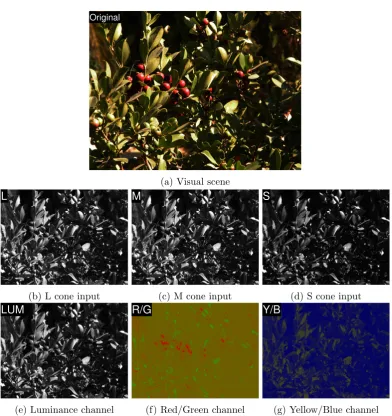
Achromatic information (or luminance) can be obtained by summing indiscriminately the three types of cones, this is a measure of light intensity as perceived by the whole

3

(28)

system. Chromatic information can be obtained by subtracting inputs, essentially decor-relating the signals by focusing on the differences between receptor outputs.4

Information transfer Photoreceptors do not spike like typical neurons in the cortex

but instead undergo modulations of their membrane potential. This potential in turn modulates the transfer of neurotransmitter (glutamate). The synapses between receptors and horizontal or bipolar cells is the second step of visual computation, and are described as post-receptoral. The effect of glutamate on horizontal and bipolar cells has been described by Shiells, Falk, and Naghshineh (1981).

Post-receptoral computation is described in the following section on interneurons and ganglion cells in the retinae, and is the basis of visual pathways. In the rest of this section on cones, I will detail some known cone deficiency to get a grasp of the role that cones are playing in visual processing. Photoreceptors are the first building blocks of perception, I will detail in the next section how some photoreceptors defects can affect perception. This will help understand their primary role.

Photoreceptor deficiency5 A subset of the population only possesses two cones; these

people are called dichromats (e.g., see Kremers et al., 2000). Dichromats have less discrim-ination for certain colours depending on the cone missing; however, it has been shown that they can detect some colour camouflaged objects better than trichromats (Morgan, Adam, & Mollon, 1992) and display other perceptual advantages (Sharpe, de Luca, Hansen, J¨agle, & Gegenfurtner, 2006). Depending on their missing cone type (L or M), more specifically missing opsin photopigment, dichromats are identified asprotanopic ordeuteranopic, re-spectively. The loci of genes, encoding for the pigment responsible for absorbing the light in cones, are on the X-chromosome. Consequently, colour perception deficiencies tend to affect more the male population. However, visual system development appears to be robust and when L or M cones are missing they seem to be replaced on the retina by the other one of the pair (Kremers, Usui, Scholl, & Sharpe, 1999).

The complete absence of a gene type (single gene dichromats) is relatively rare. Mu-tations in either gene are a more common occurrence and essentially change the peak of spectral sensitivity of the photo-pigment (Jagla, J¨agle, Hayashi, Sharpe, & Deeb, 2002; Sharpe et al., 1998). Individuals with this genotype are identified as protanomalous or as deuteranomalous and do not show the same extent of colour discrimination difficulties as protanopes and deuteranopes.

A more severe case called achromatopsia, is a case in which a person cannot distinguish colours. This can be the case if a person does not possess any cones or only the S cone type.6 Achromatopsia is also associated with other visual deficiencies, i.e. severe loss of

4_{This type of computation is more efficient than having non-overlapping narrow band receptors}

(essen-tially the colour detector describe before) as noted by Young (1802), otherwise the visual system would require a detector for each point on the retina for each shade of colour that needs to be detected.

5

Here meaning, divergence from the more frequent, ”normal”, genotype.

6

(29)

acuity.

It is well known lesion studies in neuroscience can tell us about the functionality of specific brain regions. Similarly, it is possible to study the functional role of the cones, by looking into ”abnormal” cone phenotypes. From the anomalous visual systems described previously, we can infer two main conclusions.

Firstly, several types of cones (i.e. with different light absorbance peaks) are neces-sary to perform colour discrimination. By reducing the number of cone types or shifting the absorbance peaks, discrimination is impaired. The reverse statement is also true; ex-tra cones will provide more discrimination power with appropriate neuronal processing. Tetrachromaticty (four cone types) has been hypothesized by de Vries (1948), and is still a research topic of interest (e.g. Jordan, Deeb, Bosten, & Mollon, 2010).

Secondly, the evidence shows that both L and M cone types are necessary for good performance in spatial vision, as acuity is greatly diminished whenboth are missing. How-ever, there is no lack of visual acuity in dichromats compared to trichromats (J¨agle, de Luca, Serey, Bach, & Sharpe, 2006).7 Therefore, L and M cones are crucial for spatial and chromatic perception. A complete loss of S cones (tritanopia) on its own has no effect on visual acuity (D. P. Smith, Cole, & Isaac, 1973), showing that most of the acuity is carried by L and M cone processing. I will now describe the post-receptoral processing in the following sections on intermediate neurons and ganglions cells.

2.2.2 Intermediate neurons

Dowling (1968) identified several types of cells in the retina, here I focus on one sub-group, the intermediate neurons. The intermediate neurons are composed of horizontal cells, amacrine cells, and bipolar cells.

Horizontal cells Horizontal cells and bipolar cells are in direct contact with

photore-ceptors; through their dendrites effectively forming synapses with the receptors. These synapses communicate signals using of neurotransmitters (glutamate) between cells.

Horizontal cells have dendrites aligned along the retina (hence their name) that sample larger areas of the retina than individual photoreceptors. Horizontal cells are actually modulating receptors at the centre of theirreceptive field (RF). There are possibly three types of horizontal cells (Kolb et al., 1994), named H1, H2, and H3; with different morphological properties and connectivity.

Horizontal cells are averaging the signal over space. They lose the fine grain, as the light information is pooled over a larger area of the cone mosaic, however, detection in the central cones is increased. This is done by lateral inhibition and additionally it has recently been shown that they also use central excitatory feedback in the centre cone (Jackman,

colour-discrimination (Michaelides et al., 2005).

7

(30)

Table 2.1: Bipolar cell types, IPL: Inner plexiform layer

Cell Type Characteristics ON OFF Light Centre Depolarize Polarize Light Surround Polarize Depolarize Projection IPL sublayer b IPL sublayer a

Babai, Chambers, Thoreson, & Kramer, 2011).

Bipolar cells Bipolar cells can be distinguished according to their connectivity (and

dendritic tree). They are called bipolar because of their orientation, with the dendrites facing the cones and the axon facing the outer layer of the retina.

There are two main kinds of bipolar cells: midget and parasol. Midget bipolar cells uniquely link to one photoreceptor, as discovered by Polyak (1941). Diffuse bipolar cells connect to a larger number of photoreceptors, around 6 with variations (Boycott & W¨assle, 1991). Note that there exist subgroups of these categories with morphological and con-nectivity differences (e.g. Chan, Martin, Clunas, & Gr¨unert, 2001).

These two types of bipolar cells are divided into two functional sub-types relating to their response pattern. The ON and OFF pathways emerge from these interneurons (Dacey, Packer, Diller, Brainard, & Lee, 2000). Their receptive fields are overlapping centre-surround fields of different polarity and the two populations project to two segre-gated sub-layers of the retina (see Table 2.1 and Famiglietti & Kolb, 1976; Lennie, 2003; Nelson & Kolb, 2004)

So far, I have shown that retinal processing is dependent on a combination of both horizontal cells (for contrast sharpening) and bipolar cells, through their receptor sam-pling. Connectivity in the retina after the photoreceptors has been described in detail by Kolb (1970), and more recently reviewed by Lee, Martin, and Gr¨unert (2010). The third type of intermediate interneurons, amacrine cells, seems to perform a similar role as horizontal cells, but at the layer where bipolar cells can be found, their functional role is still debated. I will therefore not discuss this subject further.8

The three types of cells I described are referred to as intermediate cells, as they are the step between photoreceptors and ganglion cells, the last type of cells on the retina identified by Dowling (1968).

2.2.3 Ganglion cells

Ganglion cells are responsible for the last stage of retinal processing. They are also re-sponsible for carrying the information to the cortex through the optic nerve. The optic

8

(31)

Position (degrees)

Sensitivity

−0.50 −0.25 0.00 0.25 0.50

1

L

[image:31.595.197.398.87.297.2]

M

Figure 2.2: Example of difference of Gaussian (DOG) model of a ganglion cell receptive field.

nerve is uniquely composed of ganglion axons. The intermediate neurons, through their horizontal connections and centre surround mechanism, play a role in determining the receptive field of the ganglion cells. The sampling strategy used by the ganglion cells in terms of connectivity (Field et al., 2010) adds to the complexity. The combination of sampling from excitatory and inhibitory interneurons and the centre-surround structure of bipolar cells provide the basis for the shape of ganglion cell receptive fields (Dacey, 2000; Dacey et al., 2000).

Ganglion cells are the precursor of sub-cortical pathways processing colour (S. G. Solomon & Lennie, 2007) and luminance signals. It is notable that the visual channels seem to match the constraints of the retinal level (Lee, 2011). The visual channels are the two colour channels L/M opponent and L,M/S opponent, roughly processing red-green and yellow-blue dimensions and the luminance channel (L+M). The terminology ”red-green” and ”yellow-blue” is slightly inadequate but widely used. It is required to have both information from L/M and L,M/S cone-opponent channels to obtain colour information (Stockman & Brainard, 2010). These psychophysical channels will be described in the next chapter. They correspond to perceptual sub-organization and are functionally (op-erationally) defined through psychophysical experiments linked to the type of signal the channels process.

(32)

Ganglion cell types

Polyak’s (1941) original description of ganglion cells divided them into two groups: midget ganglions and parasol (diffuse) cells. Midget ganglions compute the L-M signal (Dacey & Packer, 2003; Wiesel & Hubel, 1966). Parasol ganglion cells compute the luminance signal by adding several types of cones (Lee, Martin, & Valberg, 1988). Another type of ganglion cell, called bistratified, was discovered by Dacey (1993), and Dacey and Lee (1994). These three types of ganglion cells form the basis of three physiological visual pathways.

Ganglion cells tend to come in two functional types, ON and OFF, responding to the presence or absence of a stimulus. The structure of the receptive field of the retinal ganglion is thought to have a centre (either ON or OFF) and an opposite sign surround (OFF or ON, respectively), see Figure 2.2. This is referred to as connectivity opponency in the rest of this thesis. This receptive field is therefore usually modelled using adifference of Gaussian (DOG) model, (e.g. Rodieck & Stone, 1965; Sterling, 1999). However, a recent study by Field et al. (2010), which compared cone inputs to ganglion firing rates in a full retinal map, found that the smooth Gaussian was an inadequate simplification. By using a higher resolution, Field et al. (2010) found that the actual receptive field was point-like at the level of cones, or as the authors described it, ”punctate islands of light sensitivity” (p. 673), as opposed to a continuous function (Figure 2.2).

The different types of retinal ganglions and bipolar cells are the basis for the computa-tion, via parallel pathways, of selective visual aspects of the visual scene (for a full review on pathways see Dacey, 2000). The following sections describe the effect of connectivity on ganglion behaviour. The differences in these connectivity patterns are the basis for the differences in visual pathways. Note, however, that a larger number of ganglion cell types, than presented here, has been discovered (Dacey, Peterson, Robinson, & Gamlin, 2003), which might have important role to compute additional features.

Connectivity: Inputs

Midget ganglions have a single centre input from a midget bipolar (with one cone connec-tivity) (Dacey & Packer, 2003; Kolb & Dekorver, 1991). Parasol cells receive their inputs from diffuse bipolar cells with spatial pooling/averaging (Diller et al., 2004). Bistratified opponents receive an S cone input centre (Dacey & Lee, 1994), and may receive L+M surround input from horizontal cells (Dacey, 2000; Dacey & Packer, 2003).

(33)

that the ratio was determined through the intermediate cells. In turn, the ratio of inputs to the horizontal cells is supposed to be directly linked to the sampling of cones at the retina. This matches results from Dacey et al. (2000), who found that the surround of midget bipolar was probably due to horizontal cells (H1) due to the similar receptive field (RF) size.

In the periphery Diller et al. (2004) also found that midget cells summed up the inputs from L and M cones with similar ratios. They only found one cone opponent midget cell in the periphery. In contrast Field et al. (2010) found numerous colour opponent midget cells in the periphery.

Connectivity: Sampling specificity

Results by Diller et al. (2004) suggest that the variability of the L/M ratio (see Isoluminant Chapter 8) is directly linked to the variability of L/M cone distribution across the retina. The authors showed variation within but also between subjects (macaque monkeys).

In their study, Field et al. (2010) determined the connections for a wide set of ganglion cells. They found that OFF midget cells were five times more likely to sample S cones than the other types of ganglion cells, which can be linked to previous work on the S-cone OFF midget pathway by Klug, Herr, Ngo, Sterling, and Schien (2003). Conversely, parasol cells were never found to sample from S cones in accordance with findings by H. Sun, Smithson, Zaidi, and Lee (2006). The centre/surround opponency arises from a sampling bias (absolute or strong bias) in the centre but random sampling in the surround. Bistratified ganglion cells have been described to have a blue-ON receptive field (Dacey, 1993), but no opponent surround.

Connectivity: Opponency

Opponency, as introduced earlier (e.g. see Figure 2.2), is a property of neurons receiving two opposing signals to compute their outputs, with one being excitatory (or ON) the other one being suppressive (or OFF). Opponency can be, for example, achromatic, i.e. dark versus light, or chromatic, i.e. red versus green (or a composite of both). The oppo-nent process by which ganglion cells extract colour information is referred to as spectral opponency (e.g. Dacey & Packer, 2003).

(34)

input (Dacey, 2000; Dacey et al., 2000; Lee et al., 2010). Indiscriminate surround modulation can be obtained through horizontal cells (as pointed out by Dacey, 2000) and could be a good explanation for the underlying circuitry (partially confirmed by Diller et al., 2004). Furthermore, as diffuse bipolar cells receive several cone inputs in the centre, it is unlikely that the centre-surround process will generate chromatic sensitivity (Lennie, 2003).

For the case of bistratified ganglion cells, which do not possess surround suppression as pointed out in the previous section, the opponency is within the centre. The receptive field is obtained via S cone bipolar cell (ON) and the inhibition (OFF) is driven through horizontal cells (mainly pooling from L and M cones).

Separation of colour and luminance information

In terms of visual encoding, midget ganglions encode red-green colour opponency, parasol ganglions encode luminance opponency and small bistratified ganglions encode blue-yellow opponency. This section reviews how segregated these different sources of information are. The retina is the first location where there is evidence of separation of colour and luminance processing (Kaplan & Shapley, 1986). Parry et al. (2012) used a temporal compound stimulus to check the effect of luminance and colour modulation on the ERG (Electroretinogram, electrical activity measured from electrodes placed on the cornea, recording activity indiscriminately from receptors and cells, described in Section 2.2). Their temporal stimulus was designed to separate retinal pathways processing luminance and colour (red-green). They were able to distinguish the two signals showing a differential encoding of both sources of information. However, they did find differences between dichromats and trichromats, which they suggested was due to interactions between the pathways.

Lennie, Pokorny, and Smith (1993) did note the possibility that the luminance func-tion (see next chapter on Psychophysical data) could be computed from linear sums of chromatic responsive cells. Lee, Sun, and Valberg (2011) measured ganglion cell responses to luminance, chromatic (red-green and blue-yellow), and compound (chromatic at spatial frequency f and luminance at 2f) gratings. Ganglion cells (diffuse type) responded more to compound stimuli than single dimension modulations. Luminance encoding ganglion cells did respond similarly to both stimuli. However, the authors did not find any multiplexing (defined below) within the PC pathway. Lennie (2003) suggested that chromatic ganglion cells (and their projecting pathways in the cortex, i.e. the Parvocellular pathway9) might encode both colour and luminance at different temporal frequencies.

Multiplexing is a process by which two streams of information are combined into one stream containing both sources of information. It was hypothesized that the red-green channel, starting from the retina, was performing such a task (Billock, 1995; Billock & Tsou, 2004; Ingling & Martinez-Uriegas, 1983). However, the data from Lee et al.

9

(35)

(2011) suggests strict segregation of the signals (luminance and colour) from the retinal ganglion cells.

The primate’s retina is estimated to have 80 different retinal cells varying in several key characteristics. This brief review has outlined our limited knowledge of the full retinal computation. However, some main distinctive groups have been covered. The next section covers the main perceptual relay after the retina, the lateral geniculate nucleus (or LGN) of the thalamus.

2.3 LGN

The LGN is a laminar structure in the thalamus composed of six main layers (plus inter-layers that I will discuss in Section 2.3.2). It is the main relay from the retina to the cortex (Sherman & Guillery, 1996). Its structure is a direct retinotopic map (Polyak, 1957). Furthermore, as described below, it is segregated between layers of cells with different visual properties. The two main layer types are Parvocellular and Magnocellular layers carrying segregated projections from distinct ganglion cell populations.

2.3.1 Parvocellular and Magnocellular neurons

Historically two main types of layers were found, called the Parvocellular and the Mag-nocellular layers. Wiesel and Hubel (1966) classified neurons from the LGN into four categories. Type I neurons were defined by Wiesel and Hubel as chromatic opponent processing with a centre versus surround receptive field structure. Type II neurons show chromatic opponent processing but no centre-surround structure, i.e. the inhibitory and excitatory regions overlap and these cells do not provide spatial processing. However, type II were not found by Derrington and Lennie (1984).

Type III neurons have a centre-surround organisation with either excitatory or in-hibitory centre (and vice versa for the surround) and show no chromatic antagonism. Consequently, type III neurons are thought to carry the luminance information. Interest-ingly, type III’s spectral sensitivity seems to match, broadly, the photopic sensitivity, with a peak at around 550 nm. Type IV neurons showed a more complex pattern, that I will describe later on in this section.

In their study, Wiesel and Hubel (1966) acknowledged that sampling favours the upper layers (Parvocellular10) of the LGN. They managed to sample more than 200 cells from these layers compared to about thirty from the deeper layers (Magnocellular). In the Parvocellular layers they found a great majority of cells of type I (164 of 213 cells), mostly of red/green chromatic preferences (but also 3 blue-ON cells, which will be discussed in Section 2.3.2) but also some type III (34/213) luminance responsive cells. Some type II

10

(36)

cells were also found (15/213). From this, we can see that there is a clear preference in the Parvocellular layers for chromatic responsive cells. Derrington and Lennie (1984) confirmed that the Parvocellular layer mostly consists of ”spatially and chromatically opponent receptive field (type I)” (p. 237), subdivided into red-green (L-M) and yellow-blue (S- (L+M)).

In the Magnocellular layers the majority of cells found by Wiesel and Hubel (1966) were of type III (21 of 31 cells), the remaining cells they found were defined as type IV and seemed to have complex centre-surround mechanisms, very large receptive field

(RF) area, and fast non-sustained responsiveness for small spots on the RF. In general, Magnocellular layers were found to respond more to luminance patterns. Derrington and Lennie (1984) abolished the distinction between type III and IV, because they behave similarly to luminance stimuli.

Receptive fields Comparing RF size for cells of type I and III, Wiesel and Hubel

(1966) found that type III tended to have a larger RF. Therefore, it appears that there are segregated cell populations with preferential stimulus properties, i.e. chromatic or luminance, and different spatial tuning. Derrington and Lennie (1984) confirmed smaller RFs for Parvocellular (P) than Magnocellular (M) cells. Furthermore, they did not find M cells having RFs in the fovea.

Contrast sensitivity The sensitivity is low for P cells and contrast response is linear,

it is also linear for M cells but saturates at higher values (Derrington & Lennie, 1984). The contrast sensitivity, RF, and spectral sensitivity of these cells are highly linked to their pre-synaptic retinal ganglion cells. If these structures can be linked to the different retinal ganglion cell populations, then there is evidence for a physiological basis for an early separation of luminance and chromatic information from retinal ganglion cells through the LGN. Segregated projections forms separated information streams and pathways, I will discuss that point further down in the Section 2.3.3.

2.3.2 The Koniocellular pathway

A third cell population has been identified, more recently, between the Magnocellular and Parvocellular layers, which has been named Koniocellular11 (see Hendry & Reid, 2000, for a review).

It is now believed that the Koniocellular pathway consists of cells sensitive to Blue-Yellow chromatic information. Recalling some of the data of Wiesel and Hubel (1966), in their cell classification they found a couple of type I cells that they described as Blue-ON centre. Retroactively these cells can possibly be classified as part of the Koniocellular pathway.

11

(37)

Koniocellular (K) cells are composed of Blue-ON and Blue-OFF cells, sharing similar response characteristics (Szmajda, Buz´as, FitzGibbon, & Martin, 2006, although see Tailby, Solomon, & Lennie, 2008 who showed clear asymmetry between S+ and S- cells), low-pass frequency responses, and large receptive fields (compared to Parvocellular cells). As with retinal P (Parvocellular) cells (see Lee et al., 2011), K cells respond also to achromatic modulations (Szmajda et al., 2006). However, this is limited to low spatial frequency stimuli, and their response is not as high as for chromatic inputs. This double encoding (or multiplexing) was discussed in Section 2.2.3.

To summarize, the LGN is composed of three main populations of cells. These cells receive projections from the retina and, consequently, project to the primary visual cor-tex. Cells that project to the visual cortex are called relay cells (65% of all LGN cells; S. G. Solomon, 2002), as they act as a relay from the retina to the cortex, the rest are interneurons. According to the current state of our knowledge of the LGN, relay cells contribute 78% of the cells to the (4) Parvocellular layers , 10% to the (2) Magnocellular layers and 12% to the (6) Koniocellular interlayers, see S. G. Solomon (2002).

2.3.3 Retinal projections

As stated earlier, the LGN is the first relay from the retina on the path to the visual cortex. It is possible to work out the axonal projections from the projection sites in the LGN back to the retinal ganglion cells in the retina by using retrograde tracers. Leventhal, Rodieck, and Dreher (1981), used retrograde tracer12injections in Parvocellular and Magnocellular layers to find out which retinal groups projected to those layers. The authors found that Parvocellular cells had projections from midget cells and Magnocellular layers had afferent projections from parasol (diffuse) ganglions.

More recently, Szmajda, Gr¨unert, and Martin (2008) performed a similar experiment in search of the Koniocellular pathway. The injection sites for retrograde tracers tend to leak between layers and therefore are not completely localized to one layer.13 However, it is possible to determine the extent of the injection sites using histology. The data from Szmajda et al. (2008) elegantly contrasts injection site areas (between layers) and retinal cell distributions between the major known categories of retinal ganglion cells. They reproduced earlier findings showing that the Parvocellular layers mainly connect to Midget cells and a high number of Parasol cells project to the Magnocellular sites. Injection areas with a proportion of Koniocellular cells consistently increased the number of wide field (Bistratified) retinal afferent projections.

Interestingly, Szmajda et al. (2008) found that Koniocellular injection sites consistently had afferent projections from Midgets ganglions. The authors attributed these results to a different set of reasons (such as, leakage from P cells as the pipette goes through layers, easier identification and sampling of midget cells). However, as we have seen in the Retinal

12

Horseradish peroxide or RPH.

13

(38)

Section 2.2.3 there exists evidence for Blue-OFF midget cells (see Field et al., 2010; Klug et al., 2003).

The responsivity of the cells in the LGN has been determined to be due more to the direct connection from the retina than from interconnections within the LGN, first suggested by Kaplan and Shapley (1986). Consequently, the pathways are still segregated at this point of the visual processing. Due to this fact, it is now common practice to refer to the midget ganglion cells as P cells (for Parvocellular) and parasol (diffuse) ganglions as M cells. The LGN is thought to conserve the separated ON & OFF ganglion pathways (Nelson & Kolb, 2004), but this segregation disappears in the primary visual cortex.

2.4 Visual cortex

2.4.1 V1

The main projection site of the LGN is visual area 1 (V1) or striate cortex, area 17 in the macaque monkey, where most of the data presented here is from. In this section, I will detail properties of neurons in V1 related to signal processing.

LGN projections V1 has a laminar structure commonly split into six lamina (with

sub-laminae). It receives afferent connections from M and P cell mainly to layer 4C where neurons are still monocular (Hubel & Wiesel, 1977). P layer neurons project mostly to layer 4Cβ, 4A and less so to layer 6 and 1 (Lund, 1988). M layers project to layers 4Cα and less so to layer 6 (Lund, 1988). K layers (or intercalated layers in the original paper, Lund, 1988) project mostly to cytochrome oxidase-rich blobs in layer 2/3 or in the layer 4A, underneath blobs (Chatterjee & Callaway, 2003; Lund, 1988). Note that P projections in layer 4A seem to project to blobs of layer 3 as well, making blobs uniquely fit to encode chromatic information. Up to this point, it seems that the chromatic encoding pathways (P & K) and the M pathway project to separate layers (Chatterjee & Callaway, 2003). The implications for colour encoding in the cortex are addressed in the Encoding sub-section, p. 17.

Receptive fields properties Neurons in the input layer 4 are still of concentric RF just

like LGN neurons; however cells in 4Cβ are orientation selective (Livingstone & Hubel, 1984). Furthermore, most cells in other layers show orientation selectivity, with cells of similar orientation being closer to each other (Livingstone & Hubel, 1984). Probing ver-tically through the layers reveals the same orientation selectivity, thus termed orientation columns (Hubel & Wiesel, 1977).

(39)

encoded by the visual cortex are orientation and motion direction (Hubel & Wiesel, 1968). Encoding is detailed in the following sub-section.

Excitatory and inhibitory inputs to neurons change the membrane potential of the cell, which will have an effect on the firing rate of the cell and effectively shape its RF by selective sampling. In terms of contrast encoding, the behaviour of a cell related to the membrane potential is non-linear as the firing rate cannot be negative. This is modelled by using a rectification (Carandini, Heeger, & Movshon, 1997), which corresponds to a thresholding of responses.

Cells in layer 2, 3, 5 & 6 start to respond to binocular stimuli (Hubel & Wiesel, 1977), i.e. the RFs of these cells respond to stimuli presented to both eyes (not just monocular as in the LGN), encoding a similar area of the visual field. Cells in the first layer are monocular, probably due to the direct input from LGN neurons. The uppermost layer projects to higher cortical areas (extra-striate): V2 (Livingstone & Hubel, 1984), V3 and V4 (Lund, 1988).

RFs in layer 4 are smaller than in other layers (Hubel & Wiesel, 1977). Importantly, the collective RFs of V1 represent a topographic map of the visual input. Blobs are regularly spaced in this map, therefore they could provide a topographic map of chromatic information (Livingstone & Hubel, 1984).

Chromatic Encoding Initially, in their first report, Hubel and Wiesel (1968) did find

some cells (6/25 simple cells and 12/177 complex cells) responding to chromatic compo-nents. They suggested recording from ”thousands” of cells instead of hundreds to get a better sampling of cortex neurons. Hubel and Wiesel (1968) also described what are now called double opponent cells. Double opponent cells have the opponency present in both centre and surround but with the opponency reversed in the surround, e.g. red-on green-off centre and red-off green-on surround. This type of double opponent cell could be created by sampling from type II cells (with single opponency). Double opponent cells seems to be well suited for texture, form, and pattern encoding, which, Shapley and Hawken (2011) noted, are crucial for object comprehension.

(40)

The proportion of cells encoding chromatic information is greater than initially thought (Livingstone & Hubel, 1984; Poggio, Baker, Mansfield, Sillito, & Grigg, 1975; Thorell, de Valois, & Albrecht, 1984). Although current research techniques have not yet reached the sampling numbers suggested by Hubel and Wiesel (1968). Johnson, Hawken, and Shapley (2001) found few purely chromatic cells with poor orientation encoding but a large number of colour-luminance cells with strong orientation tuning (30%). Most cells were luminance encoding only (see also S. G. Solomon & Lennie, 2005). The colour-luminance cells were found especially in the layer 2/3 that projects to higher cortical areas, thus shaping the spatial processing of colour and luminance. Those colour luminance encoding cells are mostly double opponent (Johnson, Hawken, & Shapley, 2004), and have a wide range of cone weights giving a distributed encoding of colour edges (see also Lennie et al., 1990, for explanation of that phenomenon see Shapley & Hawken, 2011).

The more recent papers on colour encoding in V1 suggest a ubiquitous presence of colour neurons in V1. This was confirmed with fMRI studies in both humans’ and macaques’ V1 (Wade, Augath, Logothetis, & Wandell, 2008). The encoding of colour contrast in V1 has been shown to be dependent on the context (Wachtler, Sejnowski, & Albright, 2003), such as surround effects (see Section 2.4.3, 2.4.4 & 2.4.5). Furthermore, Wachtler et al. (2003) showed that population encoding is more representative of percep-tion than single cells. Shapley and Hawken (2011) noted that the visual system might extract hue, saturation, and brightness from a whole population of neurons.

Modular vs. multidimensional representation There is strong evidence relating

shape, form, and colour encoding (mainly Friedman et al., 2003; Lennie et al., 1990; Leventhal et al., 1995), reviewed by Shapley and Hawken (2011). Shapley and Hawken (2011) are of the opinion that the modular view of the visual brain (e.g. Livingstone & Hubel, 1988), might be inaccurate. To this effect, they cite psychophysical evidence of cross-masking between psychophysical channels (see my review in the next chapter, Section 3.4). Furthermore, they postulate a greater role of colour than just chromatic computation, i.e. the computation of reflectance vs. illumination (see Shevell & Kingdom, 2008, and next chapter).

The study of spatial interactions and the role played by chromatic information might help to uncover the computational role (as suggested by Shapley & Hawken, 2011) of some of the structures presented in this chapter. The chapter 3, on psychophysical data will emphasise the spatial processing on the computational role of the chromatic and luminance channels.

(41)

2.4.2 Contrast encoding and gain control

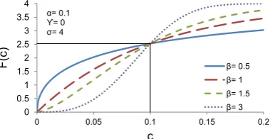
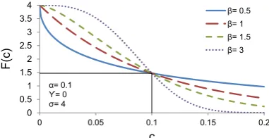
Both simple and complex cells tend to show a compressive behaviour as a function of contrast (Albrecht & Hamilton, 1982). Compressive behaviour means that the response to contrast is not linear but increases then saturates, i.e. it has a sigmoidal shape. It is usually described using the Naka and Rushton (1966) formula:

R(C) =Rmax∗(

Cn Cn₊_Cn

50

) (2.1)

In this equation, C is the contrast input, n is the rate of change, C₅₀n is the half saturation andRmax is the maximum output of the system (see Figure 2.3).

0 0.5 1 1.5 2 2.5 3

0 20 40 60 80 100

R_max=2 R_max=2.5 R_max=1.5 R_max=1

(a)Rmaxdetermines the max-imum output R.

0 0.5 1 1.5 2 2.5 3

0 20 40 60 80 100

C_50= 25 C_50= 45 C_50= 65 C_50= 85

(b) C50the semi-saturation

constant determines when

the function reaches half the maximum values(Rmax).

0 0.5 1 1.5 2 2.5 3

0 20 40 60 80 100

n= 2 n= 3 n= 5 n= 1

(c) n determines the shape of the function making it more or less steep.

Figure 2.3: Description of the Naka-Rushton equation. x axis: contrast. y axis: response strength (here arbitrary unit but can be used to fit spikes per second for example). Note that there is no parameter that forces the function to saturate before a contrast of 100.

The dynamic range is variable between neurons (Albrecht & Hamilton, 1982) so that the high slope will be found at different levels of contrast.14 Albrecht (1995) found that the semi-saturation contrast tended to be between 10% and 40% contrast (for monkey, V1 cells).

This saturating behaviour is not specific to V1 and can also be found already in the LGN. Sclar, Maunsell, and Lennie (1990) compared firing rates of LGN and V1 neurons and found that the contrast response functions become steeper and saturate faster in the cortex compared to LGN. Sclar et al. (1990) and Albrecht and Hamilton (1982) found that in general the exponent n for simple and complex cells is around 2. Increase in contrast also makes the cell respond faster (Carandini et al., 1997), this can be seen in the EEG too (Burr & Morrone, 1993).

14

(42)

2.4.3 Modulatory effects

DeAngelis, Robson, Ohzawa, and Freeman (1992) and DeAngelis, Freeman, and Ohzawa (1994) reported the distinction between two forms of suppression; one from overlay stimuli and one from purely surround effects. Surround effects (usually suppressive, but not always, e.g. Cavanaugh, Bair, & Movshon, 2002) occur when neuron RFs have a centre with driving excitatory and the surround has no driving effect but shows modulatory effects when the centre is present (DeAngelis et al., 1994, 1992; Hubel & Wiesel, 1968; Jones, Wang, & Sillito, 2002; Seri`es, Lorenceau, & Fr´egnac, 2003). Orientation selective cells will fire when presented with a stimulus in their preferred orientation and do not fire to a cross-oriented stimulus15 (Carandini et al., 1997; Kimura & Ohzawa, 2009; Morrone, Burr, & Maffei, 1982, but see also Anderson, Carandini, & Ferster, 2000). More importantly, when presented with both stimuli, preferred and cross-oriented, the contrast of the cross-oriented stimulus will have a modulatory effect on the cell response (the common effect reported is suppression; Kimura & Ohzawa, 2009; Morrone et al., 1982). Interestingly D. Xing, Shapley, Hawken, & Ringach, 2005 reported an interaction between orientation selectivity and stimulus size in V1.

The two following sections focus on these modulatory effects, the first one on overlay (cross-orientation) and the second one on modulation due to surround stimuli outside of the classical receptive field.

2.4.4 Cross-orientation effect

Masking suppression can appear when superimposing an extra grating that should oth-erwise produce no-response, to the preferred grating direction. It is thought to originate from complex cells or a group of simple cells. In some cases, the mask alone is able to activate the cell partially, in which case depending on the target contrast the mask can either enhance or suppress the response. The effect is referred to as crosstalk (Bauman & Bonds, 1991) between spatial channels.

The specificity of cross-orientation is that by itself the cross-oriented stimulus does not elicit any response from the cell. However, once the cell shows increased activity due to the presence of an optimal stimulus an additional cross-oriented stimulus drive the activity down. Priebe and Ferster (2006) studied the mechanism behind this suppressive effect in the cat’s visual cortex. The cross-orientation effects are generally thought to be cause by lateral inhibition, after receiving a broadly tuned input from the LGN. Priebe and Ferster (2006) recorded from 32 single cells in Area 17 of the cat16, using drifting gratings as stimuli. They found that the mask tended to lower the membrane potential. The non-linearity between membrane potential and spike rate amplified this effect and made the cross-orientation suppression bigger.

Interestingly, there was an interaction between test and mask contrast; at low-contrast

15

The cross-oriented case refers to the orientation relative to the best orientation±90◦.

16