On the Contribution of the Stochastic Integrals to Econometrics

(1)

https://www.scirp.org/journal/am ISSN Online: 2152-7393 ISSN Print: 2152-7385

DOI: 10.4236/am.2019.1012073 Dec. 23, 2019 1048 Applied Mathematics

On the Contribution of the Stochastic

Integrals to Econometrics

Lewis N. K. Mambo

1,2

, Rostin M. M. Mabela

3

, Isaac K. Kanyama

1,4

, Eugène M. Mbuyi

3

1_{Department of Economics, University of Kinshasa, Kinshasa, Congo}

2_{Direction of Research and Statistics, Central Bank of Congo, Kinshasa, Congo}

3_{Department of Mathematics and Computer Science, University of Kinshasa, Kinshasa, Congo}

4_{Department of Economics and Econometrics, University of Johannesburg, Johannesburg, South Africa}

Abstract

The purpose of this paper is to present the theorical connection between the Itô stochastic calculus and the Financial Econometrics. This paper has two contributions. First, we give the backgrounds on how the stochastic calculus is used to model the real data with the uncertainties. Finally, by using Con-sumer Price Index (CPI) from the Central Bank of Congo and combining the Itô stochastic calculus and the AR (1)-GARCH (1, 1) model, we estimate the stochastic volatility of inflation rate measuring efficency of monetary policy. Thus the stochastic integrals are the powerful tools of mathematical model-ling and econometric analysis.

Keywords

Stochastic Continuous-Time Models, Stochastic Volatility, AR (1)-GARCH (1, 1) Models, Inflation Rate

1. Introduction

In most dynamical systems which describe processes in economics, engineering, and physics, stochastic components and random noise are included. The sto-chastic aspects of the models are used to capture the uncertainty about the envi-ronment in which the systems are operating. For example, there are suggestions that increased uncertainty makes fiscal policy temporarily less effective [1]. Real life generates situations that require making a decision under uncertainty [2] [3] [4] [5]. By taking account of data uncertainty, the indiscriminate reduction of uncertaint observations to real numbers is avoided [5]. Uncertaint data implies

How to cite this paper: Mambo, L.N.K., Mabela, R.M.M., Kanyama, I.K. and Mbuyi, E.M. (2019) On the Contribution of the Stochastic Integrals to Econometrics. Ap-plied Mathematics, 10, 1048-1070.

https://doi.org/10.4236/am.2019.1012073 Received: October 11, 2019

Accepted: December 20, 2019 Published: December 23, 2019 Copyright © 2019 by author(s) and Scientific Research Publishing Inc. This work is licensed under the Creative Commons Attribution International License (CC BY 4.0).

http://creativecommons.org/licenses/by/4.0/

(2)

DOI: 10.4236/am.2019.1012073 1049 Applied Mathematics

information exhibiting inaccuracy, uncertainty and questionability [5]. The ma-thematical modeling of the uncertainty in economics and finance can be found in [2] [3] [5]-[12].

Therefore, the stochastic state space models and time series analysis have been both intensively and extensively developed during the past twenty years. A uni-fied theory has been constructed during this period and the concepts and me-thods have been widely applied to problems in the area of engineering and communication, economics and management. Because of these developments, interest in stochastic state space model and its applications has greatly increased in econometric research.

This paper presents the stochastic integrals and numerics which permit suc-cessful mathematical modelling not only in econometrics but also in many other fields such biometrics, psychometrics, environment science, and hydrology, as-suming of course that a suitable sequence of observed data is available.

For estimating the parameters of both stochastic continuous and discrete-time models, the methods of maximum likelihood are usually used by researchers be-cause of its capacity to give the best unbaised estimators [9] [13] [14] [15] [16] [17].

The purpose of this paper is to emphasize on the linkage between the theory of stochastic integrals and time series analysis used in the econometric analysis

[6] [16] [18] [19] [20] [21]. The stochastic integrals and numerics are considered as bridges that link the stochastic continuous-time models and the discrete time models [14] [18] [22] [23] [24] [25].

The structure of the paper is as follows. In Section 2 we will give the theory of stochastic integrals that is usefull to economic analysis. In Section 3 we give some stochastic differential equations used as econometric models that are used to express the economic theories. Section 4 gives some numerical methods to perform the empirical analysis. Section 5 illustrates the use of the stochastic in-tegrals to time series econometric by estimating the stochastic volatility from the Autoregressive-Generalized Autoregressive Concoditional Heteroskedasticity model, that is, AR (1)-GARCH (1, 1) model.

2. Stochastic Integrals

Since the works of Kuyosi Itô the field of stochastic integrals attract the attention of many mathematicians and researchers [19] [26]-[33].

Itô Stochastic Integrals developed here are from [28] [29] [34] [35].

Definition 2.0.1 A process X is called adapted to the filtration (t), if for all t,

( )

X t is t-measurable.

Proposition 2.0.1. (a) X =

( )

Xt , where Xt is a d-dimensional measurable,

t

 -adapted process is a continuous semimartingale if

X

t is continuous and

has the form

0

t = + t+ t

(3)

for all t (a.s.), where E X0 < ∞, (1) M =

( )

Mt is a continuous

2

L -t

-martinagle with M0=0 (a.s.) and (2)

( )

Bt ∈.

(b) If in the decompostion 1, (Mt), is a continuous local martingale and (Bt)

belongs to



loc, then (Xt) will be called a continuous local semi-martingale.

Theorem 2.1. [35] [36] Let X t

( )

be a regular adapted process such that

with probability one 2

( )

0 d

T

X t t< ∞

∫

. Then Itô integral

∫

₀TX t

( ) ( )

dB t is

de-fined and has the following properties:

1) Linearity. If Ito integrals of X t

( )

and Y t

( )

are defined and α and β

are some constants then

( )

(

)

( )

( ) ( )

0 d 0 d 0 d .

T T T

X t Y t B t X t B t Y t B t

α +β =α +β

∫

(2)

2) ₀

( )

( ,]

( ) ( )

d

( ) ( )

d

T b

a b _a

X t I t B t = X t B t

∫

. The following two properties hold when the process satisfies an additional assumption

( )

(

2

)

0 d .

T

E X t t< ∞

∫

(3) 3) Zero mean property. If condition 3 holds then

( ) ( )

(

0 d

)

0,

T

E

∫

X t B t =

(4) where E denotes expectation with respect to classical Wiener measure.

4) Isometry property. If condition 3 holds. Then

( ) ( )

(

)

2 2

( ) ( )

0 d 0 d

T T

E

∫

X t B t =E

∫

X t B t

(5) Corollary 2.1.1. If X is a continuous adapted process then the Itô integral

( ) ( )

0 d

T

X t B t

∫

exists. In particular,

∫

₀Tf B t

(

( )

)

dB t

( )

where f is a continuous

function on R is well defined.

A consequence of the isometry property is the expectation of the product of two Itô integrals as given in the following theorem.

Theorem 2.2. [36] Let X t

( )

and Y t

( )

be regular adapted processes, such

that

( )

2

0 d

T

X t t< ∞

∫

and

( )

2 0

T

Y t < ∞

∫

. Then

( ) ( )

(

₀T d ₀T d

)

₀T

(

( ) ( )

)

d .

E

∫

X t B t

∫

Y t B t =

∫

E X t Y t t

(6) where E denotes mathematical expectation.

We denote by _mn_{all real-valued}

m n× matrices and by

( )

(

1

( )

, , n

( )

)

, 0. W t = W t W t ′ t≥

Let

[ ] [ [

a b, ∈ 0,∞ and we put

[ ]

(

,

)

{

:

[ ]

, mn| 1 , 1 :

(

[ ]

,

)

}

,

W ij Wj

C a b = f a b × Ω → ∀ ≤ ≤i m∀ ≤ ≤j n f ∈C a b

[ ]

(

,

)

{

:

[ ]

, mn| 1 , 1 :

(

[ ]

,

)

}

IW ij IWj

C a b = f a b × Ω → ∀ ≤ ≤i m∀ ≤ ≤j n f ∈C a b

and C_I

(

[ ]

a b,

)

respectively.

(4)

the stochastic integral with respect to W is the m-dimensional vector defined by

( )

1 ₁ d d n b b ij j a a

j _{i m}

f t W t f t W t

= _{≤ ≤} ′   =   

∑



∫

(7)

where each of the integrals on the right-hand side is defined in the sense of Itô. Proposition 2.2.1. (Itô formula) [36] [38] Let Xt=X0+Mt+Bt be a

d-dimensional continuous semimartingale. Let 2

( )

d b

F∈C  , that is, let

: d

F  → be bounded and continuous and have bounded, continuous

deriva-tives of orders 1 and 2. Then,

( )

0 ₀ ₀

0 0 2 0 0 d d 1 d , 2

d _t d _t

i i

t i s s i s s

i i

d _t

i j

s

i j _s

i

F F

F X F X X M X B

x x

F

X M M

x x = = = ∂ ∂ = + + ∂ ∂ ∂ + ∂ ∂

∑

∫

∑

∫

∑∫

(8)

Stratonovich Stochastic Integrals. In [39], the multidimensional Stratono-vich integrals Sm

( )

f can be expressed by the following formula using Itô

in-tegrals

( )

₍

₎

2

(

)

2

!

. 2 ! 2

k

m k m k

k

m

S f I Tr f

k m k −

≤

=

−

∑

(9)

where Tr denoted the iterated traces that are defined formally starting with

(

1, , m 2

)

(

1, , m 2, ,

)

d .

Trf s  s − =

∫

f s  s − s s s

Another approach to formula (9) using Hida’s theory of white noise. Working on _m instead of m

+

 and assuming that f is a test-function, the integral

( )

m

S f may indead be rewritten as

(

1, ,

)

₁

( )

d1 d

,

m

m s s n

n

f s s X w X w s s

f X⊗

=

∫

_  _  _



where the derivative of Brownian motion is understood in the distribution sense. In the sense of Hu and Meyer [39], a Stratonovich integral is given in rigorous form as

( )

_{[ )}

(

1

)

1

( )

1

, , d d ! S m m s sm m

S f f s s X w X w

m

=

∑ ∫

 

(10) where f is a finite sequence of coefficients 2

( )

m

m s

f ∈L 

and n!= × − × ×n

(

n 1

)

 1.

Itô’s Formula for Functions of Two Variables. If two processes X and Y both possess a stochastic differential with respect to and f x y

(

,

)

has

conti-nuous partial derivatives up to order two, then f X t Y t

(

( ) ( )

,

)

also possesses a

stochastic differential.

Theorem 2.3. [36] Let f x y

(

,

)

have continuous partial derivatives up to

order two (a 2

(5)

( ) ( )

(

)

(

( ) ( )

)

( )

(

( ) ( )

)

( )

( ) ( )

(

)

(

( )

)

( ) ( )

(

)

(

( )

)

( ) ( )

(

)

(

( )

)

(

( )

)

2

2 2

2

2 2

2

d , , d , d

1

, d

2 1

, d

2

, d

X

Y

X Y

f f

f X t Y t X t Y t X t X t Y t Y t

x y

f

X t Y t X t t

x f

X t Y t Y t t

y

f

X t Y t X t Y t t

x y

σ

σ σ

∂ ∂

= +

∂ ∂

∂ +

∂ ∂ +

∂ ∂

(11)

An important case of Itô formula is for functions of the form f X t t

(

( )

,

)

.

Theorem 2.4. [29] [36] [40] Let f x t

( )

, be twice continuously differentiable

in x, and continuously differentiable in t (a 2,1

C function) and x be an Itô

process, then

( ) ( )

(

)

(

( ) ( )

)

( )

( ) ( )

(

)

( )

(

)

2

(

( )

)

2

d , , d , d

1

, , d 2 X

f f

f X t Y t X t Y t X t X t X t t t

x t

f

X t t X t t t x

σ

∂ ∂

= +

∂ ∂

∂ +

∂

(12)

Stochastic Calculus. Let

(

1 2

)

2 , , , n

f x x  x ∈C and

(

1 2

)

, , , n

X X  X ∈Q

and

(

1 2

)

, , , n

Y= f X X  X ∈Q. We denote by Q the totality of

quasimartin-gales.

Definition 2.4.1. [36] For X Y, ∈Q, we say that X and Y are equivalent and

write X Y if, with probability one,

( )

X t −X s =Y t −Y s for every

0 ≤ ≤

s

t

.

The equivalence class containing X is denoted by dX and is called the stochas-tic differential of X. As known, by definition,

( )

d

t

s X u

∫

is the process X t

( )

−X s

( )

.

Let dQ=

{

d ;X X∈Q

}

, dM =

{

dM M; ∈M

}

and dA=

{

d ;A A∈A

}

. We

in-troduce the following operations in dQ [36].

(1) Addition: dX+dY =d

(

X+Y

)

for X Y, ∈Q.

(2) Product: dX⋅dY =d M Mx, y for X Y, ∈Q where Mx and My are

the martingale parts of X and i respectively.

(3) B-multiplication: If Φ ∈B and X∈Q, then

(

Φ ⋅X

)

= X

( )

0 + Φ

∫

₀t

(

s w,

)

dMx

( )

s + Φ

∫

₀t

(

s w A,

) ( )

x s t, ≥0

is defined as an element in Q. Hence d

(

Φ ⋅X

)

is defined from Φ and dX.

We define an element Φ ⋅dX of dQ by Φ ⋅dX =d

(

Φ ⋅X

)

.

Theorem 2.5. [36] The space dQ with the operations (1), (2) and (3) is a commutative algebra over B, i.e., a commutative ring with the operations (1) and (2) satisfying the relations

(a) Φ ⋅

(

dX+dY

)

= Φ ⋅dX + Φ ⋅dY ,

(b) Φ ⋅

(

dX⋅dY

) (

= Φ ⋅dX

)

⋅dY ,

(6)

(d)

(

Φ ⋅ Ψ ⋅

)

dX = Φ ⋅ Ψ ⋅

( )

dX,

for Φ Ψ ∈, B and d , dX Y∈Q. We also have that dQ⋅dQ∈dA, dQ⋅dA=0

and dQ⋅dQ⋅dQ=0.

If

(

1 2

)

, , , n

X X  X ∈Q and 2

f ∈C , then Y = f X

(

1,X2,,Xn

)

∈Q and

(

)

(

)

1 , 1

1

d d d d .

2

d d

i i j

i i j

Y f X f X X

= =

=

∑

∂ ⋅ +

∑

∂ ∂ ⋅ ⋅

(13) where ∂if and ∂ ∂i jf are elements in B defined by

(

)

1 2 , , , d i

f

X X X

x

∂

∂ 

and

(

1 2

)

, , , d

i j f

X X X

x x

∂

∂ ∂  , respectively. If

1 2

d_X , d_X ,_, d_Xd∈d_M_and

dXi⋅dXj =

δ

ijdt, i j, =1, 2,,d then

(

( )

)

1 2

, , , d

X t X t  X t is a

d-dimensional Wiener process. Such a system of martingales

(

1 2

)

, , , n

X X  X

is called a d-dimensional Wiener martingale. (4) Symmetric Q-Multiplication

1

d d d d

2

Y X = ⋅Y X+ X⋅ Y or dX∈dQ and Y∈Q

Theorem 2.6. [35] [36] The space dQ with the operations (1), (2), (3) and (4) is a commutative algebra over Q; we have for X Y Z, , ∈Q,

(

d d

)

d d ,

X Y+ Z =X Y+X Z

(

X+Y

)

dX =XdZ+Yd ,Z

(

d d

) (

d

)

d

(

d d

)

,

X Y⋅ Z = X Y ⋅ Z =X⋅ Y⋅ Z

(

X Y⋅

)

dZ =X 

(

Y dZ

)

.

where  denotes Stratonovich product. Theorem 2.7. If

(

1 2

)

, , , n

X X  X ∈Q and 3

f ∈C , then for

(

1 2

)

, , , n

Y = f X X  X ∈Q we have

1

d d .

d

i i i

Y f X

=

∑

∂ 

(14) The stochastic integral

∫

₀tYdX is called the Stratonovich integral or the

Fisk integral or sometimes the Fisk-Stratonovich symmetric integral. Indeed, we have the following theorem:

Theorem 2.8. [36] For every X and Y in Q,

( ) ( ) ( ) ( )

1

(

)

1 0

1

d . . . , 0,

2

n

t _i _i

i i

i

Y t Y t

Y X l i p − X t X t−

=

−

=

∑

− ∆ →

∫



(15) where ∆ denotes a partition 0= < <t0 t1 < =tn 0 and

(

1

)

max ti ti−

∆ = − _,

1 ≤ ≤

i

n

.

Skorokhod Integral. The Skorohod integral is an extension of the Itô integral to non-adapted processes and is the adjoint of the Malliavin derivative, which is fundamentals to the stochastic calculus of variations [41] [42].

(7)

(

)

_{( )}

1

2 0

ˆ

1 ! _n _n .

n

n f ₊

∞

=

+ < ∞

∑

_

(16) Then we define the Skorohod integral of Y t

( )

denoted by

( ) ( )

,

Y t

δ

B t

∫



by

( ) ( )

(

)

( )

₍

₎

1

1 1 1 1

0

, , d , , .

n

n n n

n

Y t δB t + f s s B s s

∞

⊗ +

+ +

=

∑∫

_  

(17) where

⊗

_{represents the Kronecker product.}

Wick Product. The Wick product was introduced in Wick (1950) as a tool to renormalize certaint infinite quantities in quantum field theory. In stochastic analysis the Wick product was first introduced by Hida and Ikeda (1995). The Wick product is important in the study of stochastic differential equations. In general, one can say that the use of this product corresponds to and extends na-turally—the use of the Itô integrals. The Wick product can be defined in the fol-lowing way:

Definition 2.8.2. The Wick product F◊G of to elements

( )

:

1

, m N

H

α α α α

α α −

=

∑

=

∑

∈

F a G b H S

(18) with a b_α, _α∈N is defined by

(

)

,

α β α β

α β +

◊ =

∑

F G a b H

(19) In the 2

( )

µ

L cas the basis independence of the Wick product can be seen from the following formulation of Wick multiplication in terms of multiple Itô integrals.

Proposition 2.8.1. Let N= = =m d 1. Assume that f g, ∈L2

( )

µ

have the following representation in terms of multiple Itô integrals:

( )

0 0

d , d ,

i j

f w f B g w g B

∞ ∞

⊗ ⊗

= =

=

∑

_∫

=

∑

_∫

 

(20) Suppose _{◊ ∈} 2

( )

µ

F G L . Then

( )

0

ˆ _d _.

n

i j

i i j n

f w B

∞

⊗

= + =

=

∑ ∑

_∫

⊗

 f g

(21) For the relation between the Wick multiplication and The Itô-Skorohod Inte-gration we put N= = =m d 1 for simplicity. One of the most stricking features

of the Wick product is its relation to Itô-Skorokhod Integration. In short, this relation can be expressed as

( ) ( )

( )

d .

nY t

δ

B t = nY t ◊W t t

∫



∫

 (22)

Here the left hand side denotes the Skorokhod integral of the Stochastic process Y t

( )

=Y t w

( )

, (which coincides with the Itô integral if Y t

( )

is

adapted), while the right hand side is to be interpreted as an

( )

*

S -valued (Pettis)

(8)

im-DOI: 10.4236/am.2019.1012073 1055 Applied Mathematics

portnat in stochastic calculus.

3. Stochastic Differential Equations Models

The objective of this section presents in short the two main types of stochastic differential equation models. The theory of stochastic differential equation is very vaste and well known by Engineers and other scientists but less known and understood among economists. For further reading the reader can see [36] [43]-[48].

Example 1: Stochastic Differential Equation Model. Let X

( )

t be a

diffu-sion in n dimensions described by the multidimensional stochastic differential equation

( )

(

( )

)

(

( )

)

( )

dX t = Φ X t t, dt+ Ψ X t t, dB t ,

(23) where Ψ is n d× matrix valued function, B is d-dimensional Brownian

motion and and X and Φ_aren_{-dimensional vector valued functions. The}

vector Φ

( )

X,t and the matrix Ψ

( )

X,t are the coefficients of the stochastic

differential equation.

Theorem 3.1. [34] (Uniqueness and Existence of Solution) If the coeffi-cients are locally Lipschitz in X with a constant independent of t; that is, for every N, there is a constant K depending only on T and N such that for all

,

x y ≤N and all

0 ≤ ≤

t

T

,

( )

,t

( )

,t

( )

,t

( )

,t K ,

Φ x − Φ y + Ψ x − Ψ y ≤ x y−

(24) for any given X

( )

0 the strong solution to stochastic differentional Equation

(27) is unique. If in addition to condition 24 the linear growth condition holds

( )

,t

( )

,t K_τ

(

1

)

,

Φ x + Ψ x ≤ +x

(25)

( )

0

X is independent of B, and E X

( )

0 2 < ∞, then the strong solution

ex-ists and is unique on

[ ]

0,T , moreover,

( )

(

2

)

(

( )

2

)

sup t <C 1+E 0 ,

E X X

where the constant C depends only on K and T.

The following theorem gives the solution of stochastic differential equations as Markov processes.

Theorem 3.2. [34] (The solution of SDEs as Markov processes) If equation 27 satisfies the conditions of the existence and uniqueness theorem 3.1, the solu-tion Xt of the equation for arbitrary initial values is a Markov process on the

interval

[

t T0,

]

whose initial probability distribution at the instant to is the

dis-tribution of C and whose transition probabilities are given by

(

, ,t

)

(

t | s

)

(

t

( )

,

)

P s x B =P X ∈B X =x =P X s x ∈B

(26) where Xt

( )

s x, is the solution of equation.

(9)

( )

(

( )

)

(

( )

)

( )

0 0

dX t = Φ X t t, dt+ Ψ X t t, dB t ,Xt =C,t ≤ ≤t T,(27)

where d t

X ∈R , Φ

( )

t x, ∈Rd, m

B∈R and Ψ

( )

t x, is a d m× matrix. If in

addition, the functions Φ and Ψ are continuous with respect to t, the

solu-tion Xt is a d-dimensional diffusion process on

[

t T0,

]

with drift vector and

diffusion matrix Π

( )

t x, = Ψ

( ) ( )

t x; Ψ t x, ′. In particular, the solution of an

au-tonomous SDE is always a homogeneous diffusion process on

[

t0,∞

)

.

Example 2: Differential Equation with Markovian Switching Model. For economists, the economic phenomena can be governed by uncertainties and cycles. This model was developped by [49] as hybrid models. Consider the Sto-chastic Differential Equation with Markovian Switching of the form

( )

(

( ) ( )

)

(

( ) ( )

)

( )

dY t = f Y t ,R t dt+g Y t ,R t dW t , t≥0.

(28) Here the state vector has two components: Y t

( )

and R t

( )

. The first one is

normally referred to as the state while the second one is regarded as the mode. In its operation, the system will switch from one mode to another in random way, and the switching among the modes governed by the Markov chain R t

( )

.

Example 3: Differential with Respect to Fractional Brownian Motion Model. Let B=

{

Bt,t≥0

}

be a m-dimensional fractional Brownian motion of

Hurst parameter H∈

(

1 2 ,1

)

. This means that the components of B are

inde-pendent fractional Brownian motions with the same Hurst parameter H. For further reading see [46] [50] [51].

Consider the equation on m

(

)

(

)

[ ]

0 ₀ ₀

1

, d , d , 0, ,

m

t _j t

t j s s s

j

s B s s t T

σ φ

=

= +

∑∫

_ +

_∫

∈

x x x x

(29) where x0 is an m-dimensional random variable.

Assumption 3.3.1. Let us introduce the following assumptions on the coeffi-cients:

A1. σ

( )

t,x is differentiable in x, and there exists some constants 0<β δ, ≤1

and for every

N

≥

0

there exist MN >0 such that the following properties

hold:

( ) ( )

, , 0 , ,

[ ]

0, ,

m

t x t y M x y x t T

σ

−

φ

≤ − ∀ ∈_ ∀ ∈

( )

,

( )

, 0 , , ,

[ ]

0, ,

i i

m

x t x x t y M x y x y t T

δ

σ

φ

∂ − ∂ ≤ − ∀ ∈_ ∀ ∈

( ) ( )

t x, t y, xi

( )

t x, xi

( )

t y, M t0 s ,

β

σ

−

φ

+ ∂

σ

− ∂

φ

≤ −

A2. The coefficient φ

( )

t x, satisfies for every

N

≥

0 ( ) ( )

t x, t y, L x_N y, x y, N, t

[ ]

0,T ,

φ

−

φ

≤ − ∀ ≤ ∀ ∈

( )

, 0 0

( )

, ,

[ ]

0, ,

m

t x L x t x t T

φ

≤ +

φ

∀ ∈ ∀ ∈

where 0

(

0, ;

)

p m

L T

φ

∈  ), with ρ≥2 and for some constant LN >0.

Consider the stochastic differential equation with respect to fBm (29) on m

(10)

and X0 is an m-dimensional random variable.

Suppose that the coefficients

σ φ

j, i:Ω×

[ ]

0,T ×m → are measurable

functions satisfying conditions A1 and A2, where the constants MN and LN

may depend on

ω ∈Ω

, and β > −1 H , 1 1

H

δ > − _{. Fix}α _{such that}

0

1 1 min , ,

2 1

H α α β δ

δ

 

− < < = _ _

+

  a uniue continuous solution such that

( )

, 0 0,

i

X ∈Wα ∞ T for all i=1, 2,,m. Moreover the solution is Holder

conti-nuous of order

1 −

α

.

Example 4: Differential Equation with Jumps Models. In real world, some phenomena or economic policy decisions are governed under uncertainty with jumps. Therefore, stochastic differential equation with jumps modeling can be considered as a usefull econometric approach [32]. Consider a one-dimensional SDE, d = 1, in the form

(

)

(

)

(

) (

)

dX_t a t X, _t dt b t X, _t dW_t c t X, _t ,v p_ϕ d , dv t

ε −

= + +

_∫

(30) for t∈

[ ]

0,T , with X0∈ , and W=

{

W tt, ∈

[ ]

0,T

}

an t -adapted

one-dimensional Wiener process. We assume an an t-adapted Poisson

meas-ure p_ϕ

(

d , dv t

)

with mark space ε ⊆\ 0

{ }

and with intensity measure

( )

dv dt F

( )

dv dt

ϕ =λ _{, where}F

( )

. is a given probability distribution function

for the realizations of the marks. Consider a one-dimensional SDE with Jumps (30) in integral form, is of the form

(

)

(

)

( )

(

)

0 ₀ ₀

1

, d , d , _i

p t

t t

t s s s i

i

X X a s X s b s X W c X

ϕ

τ

=

= +

_∫

+

_∫

+

∑

(31) Example 5: Partial Differential Equation Models. Stochastic Partial Diffe-rential Equation Models are used as power tools of mathematical modeling in many areas [52] [53] [54].

Consider the Itô Stochastic Partial Differential Equation of the form as men-tioned in [27]

( )

dXt=AXt+F Xt dt+B Xt dWt, Xt_∂_ =0,X=

ξ

(32) for

t

≥

0

, where W_t, is an infinite dimensional Wiener process of the form

(

)

( ) ( )

1

, j , 0,

t j t j

j

W x w C W w φ x t x

∞

=

∑

≥ ∈

(33) with independent scalar Wiener processes j

t

W , j∈ and. Note that

A= ∆ (Laplacian with Dirichlet boundary conditions) and B U

( )

≡I in one

spatial dimension has sample paths which are only 1

4 ε

 ₋ 

 

 -Hölder continuous.

Here the family

φ

j, j∈, is an orthonormal basis in,

(

)

2 , 

L .

Assumption 3.3.2. [27] (1) Linear operator A. Let



be a finite or countable set. In addition, let

( )

λ

i i∈ be a family of real numbers with infi∈ > −∞ and

(11)

is given by Aυ=

∑

i=−λ ϑ υ ϑi, i for all υ ∈

( )

A with

( )

{

2 2

}

,

i i

A =

∑

₌_λ ϑ υ ∈H

 . (2) Drift term F. Let

α δ

, ∈ be real

num-bers with

δ α

− <

1

and let F H: δ →Hα be a globally Lipschitz continuous

mapping. (3) Diffusion term B. Let

α δ

, ∈ be real numbers with 1 2

δ β− <

and let F H: δ →HS

(

υ

0,Hβ

)

be a globally Lipschitz continuous mapping. (4)

Initial value ξ: Let

γ

∈_

δ

, min

(

α

+1,

β

+1 2

)

_ and p∈

[

2,∞

)

be real

num-bers and let

ξ

:Ω →H_γ be an  ₀

( )

H_γ -measurable mapping with

p Hγ

ξ

 _{ < ∞}

 

 

E .

The literature contains many existence and uniqueness theorems for mild so-lutions of SPDEs. Theorem below provides an existence, uniqueness, and regu-larity result for solutions of SPDEs with globally Lipschitz continuous coeffi-cients in the Equation (32).

Theorem 3.4. [27] Let Assumptions 3.3.2 (1)-(4) be fulfilled. Then there exists a unique of the Equation (32) that is predictable stochastic process

[ ]

: 0,T × Ω →H_γ

X satisfying sup p

Hγ

ξ

 _{ < ∞}

 

 

E and

( )

_{( )}

( )

_{( )}

0 0

e t te t s d te t s d

t ξ s s Xs s

− −

= A +

_∫

A +

_∫

A

X F X B W

(34)

. .

a s

−



for all t∈

[ ]

0,T . In addition,

( , ] min( ,1 2)

(

[ ]

0, ,

(

,

)

r p

r

r C T H

γ

γ −

∈ −∞

∈_ Ω

X L .

4. Numerical Methods for Stochastic Differential Equations

In this section we give a brief review some numerical methods used in the sto-chastic analysis that can be usefull for economists and social scientists. These main books can help econometricians and economists to improve and under-stand the numerical methods for stochastic analysis [27] [45] [55]-[61]. The numerical methods for stochastic ordinary differential equations can be summa-rized as follows.

The Euler-Maruyama Scheme. We consider a scalar Itô stochastic ordinary differential equation (SODE) [27]

( )

dxt = f t x, t dt+g t x, t dWt (35)

with a standard scalar Wiener process W tt, ≥0. The SODE (35) is in fact a

symbolic representation for the stochastic integral equation

(

)

(

)

0 ₀ , d ₀ , d

t t

t t _t t _t t t

x =x +

∫

f t x t+

∫

g t x W

(36)

The simplest numerical scheme for the SODE (35) is the Euler-Maruyama Scheme given by

(

)

1

(

)

1

1 , d , d

n n

t t

n n n n _t n n _t s

Y₊ =Y + f t Y

∫

+ s+g t Y

∫

+ W

(12)

where one usually writes

1 1

d , d ,

n n

t t

n _t s Wn _t Ws

+ +

∆ =

_∫

∆ =

_∫

for n=0,1,,MT −1 and where t0 < <t1 <tM =T with MT∈ is an

ar-bitrary partition of

[

t T0,

]

.

The Milstein Scheme [27]. The another useful numerical scheme for the SODE (35) is the Milstein Scheme given by

(

)

(

)

(

) (

)

1 1

1

1 , d , d

, , d d

n n

n

n n

t t

n n n n _t n n _t s

t s

n n n n _t _t u s

Y Y f t Y s g t Y W

g

g t Y t Y W W

x + + + + = + + ∂ + ∂

∫

∫ ∫

(38)

Numerical Methods for Stochastic Differential Equations with Jumps. The Euler scheme for SDE with jumps (30), is given by the algorithm [32] [62] [63],

( ) (

)

1

1 d , d

n

n t

n n n n _t

Y+ =y + ∆ + ∆a b W +

∫ ∫

+ _εc v pϕ v z

( ) ( )

( )

1 1 1 n p t

n n n n i

i p t

Y Y a b W c

ϕ ϕ ξ + + = + = + ∆ + ∆ +

∑

(39)

for n∈

{

0,1,,N−1

}

with initial value Y0 =X0. Here ∆ =n tn+1−tn is the

length of the time interval

[

t tn, n+1

]

and ∆Wn=Wt_n+₁−Wt_n is the n

th_Gaussian

(

0, n

)

N ∆ distributed increment of the Wiener process W, n∈

{

0,1,,N−1

}

,

( )

(

, 0,

[ ]

)

p_ϕ t = p_ϕ

ε

t represents the total number of jumps of Poisson random

measure up to time t, which is Poisson distributed with mean

λ

t

.

In the multidimensional case with mark-indepedent jump size we obtain the kth_{component of the Euler scheme}

( ) ( 1)

, 1

1

n

p t

k k k k j k

n n n n n

i p t

p ϕ ϕ + + = + = + ∆ +

∑

∆ + ∆

Y Y Y b W c

(40) Methods for Stochastic Partial Differential Equations. This material is from [64]

( ) (

) ( )

(

) (

(

) ( )

( )

(

)

(

( )

)

( )

)

(

) (

(

) ( )

( )

(

)

(

( )

)

( )

)

( )

1 1

1 1 1

1

d d d

n j n j n n j j n j n j n n j j t

n n n n n n n

j j j j _t j j j

s s

t t

t _n _n _n

j j j

t

s s

t t

X t S t t X t S t s B S s t x t

Bx r r S s r G x r M r s

S t s B S s t X t

BX r r S s r G x r M r M s

+ + + + + + = − + − − + + − + − − + + −

∫

(41)

Methods for SPDE with Multiplicative Noise. Two representative numerical schemes used in the literature for the Stochastic Partial Differential Equation (32) are the linear-implicit Euler and the linear-implicit Crank-Nicolson schemes

[27].

(13)

(

)

(

)

(

)

(

)

1

, , , , , ,

1 1 1

1 , ,

, 1 , . .

N M L N M L N M L

k N k N k

N M L

N N L k k

Y I hA Y hF Y

I hA B Y W a s

−

+ + +

−

+

= − +

+ − ∆ −

(42)

The Crank-Nicolson scheme

(

)

(

)

1

, , , , , ,

1 1 1

1

, , ,

2 2

, . . 2

N M L N M L N M L

k N N k N k

N M L

N N L k k

h h

Y I A I A Y hF Y

h

I A B Y W a s

−

+ + +

−

 

   

=_ − _ __ + _ + _

    

 

+_ − _ ∆ −

  

(43)

for k∈

{

0,1,,M−1

}

and N M L, , ∈. Here it is necessary to assume that

0 λ ≥

for all

i

∈



in Assumptions 2 in order to ensure that

(

I−hA

)

is

in-versible for every h≥0.

Convergence of SPDE with Multiplicative Noise. The convergence of the exponential Euler scheme will proved under the following assumptions.

Assumption 4.0.1. (A5) (Linear operator A). there exist sequences of real ei-genvalues 0<λ1≤λ2< and orthonormal eigenfunctions

( )

en n≥1 of −A

such that the linear operator A D A:

( )

∈H→H is given by

1

, ,

n n n

Av λ e v

∞

=

∑

−

for all v∈D A

( )

with

( )

{

: ₁ _n2 _n, 2

}

n

D A = v∈H

∑

∞₌ λ e v < ∞ .

(A6) (nonlinearity of F). The nonlinearity

F H

:

→

H

is two times

conti-nuously Fréchet differentiable and its derivatives satisfy the following conditions

( )

_H,

F x′ −F′ y ≤L x−y

( )

_{( )( )}

,

r r

H H

A − − F x′ A v L v

− − ≤

for all x y, ∈H, v∈D

(

( )

−A r

)

, and r=0,1 2 ,1, and

( )(

)

( )

1 2

( )

1 2

1 _, _,

H H

A F− ′′ x v w ≤L −A − v −A − w

for all x y, ∈H, where

L

>

0

is a positive constant.

Let Q be a nonnegative definite symmetric trace-class operator on a separable Hilbert space K,

{ }

fj _j₁

∞

= be an ONB in K diagonalizing Q, and let the

corres-poing eigenvalues be

{ }

1

j _j

λ ∞

= . Let

{

w tj

( )

}

t≥0, j=1, 2,, be a sequence of

inde-pendent Brownian motion defined on filtered probability space

(

Ω, ,

{ }

t _t,P

)

.

The process 1 2 1

t j j j j

w =

∑

∞₌λ w f is called a Q-Wiener process in K.

(A7) (Cylindrical Q-Wiener process Wt) There exist a sequence

( )

qn n≥1 of

positive real numbers and a real number γ ∈

( )

0,1 such that

2 1 1

n n

n

q

γ

λ ∞

−

=

< ∞

∑

and pairwise independent scalar t -adapted Wiener process

( )

Wt t≥0 for

1

(14)

1

.

n

t n t n

n

W q W e

∞

=

∑

(44) (A8) (Initial value). The random variable x0: D

(

( )

A

)

γ

Ω → − satisfies

( )

4 0

H

A γx

− < ∞

E , where γ >0 is given in A7.

The convergence theorem for SPDE model 32

Theorem 4.1. (Convergence Theorem [27]) Suppose that Assumptions 3 (A5)-(A8) are satisfied. Then there is a constant CT >0 such that

( )

1 2 ₂ , 0, ,

log

sup ,

k

N M

t k T N

H

k M

M

X Y C

M

γ

λ− =

 

 ₋  _≤ ₊

   

  _ _

  (45)

holds for all N M, ∈, where X_t is the solution of SPDE 32, Yk(N M, ) is the

numerical solution given by 42, k k

t T

M

= _for k=0,1,,M, and γ >0 is the

constant given in Assumption A8.

5. Application to Stochastic Volatility Estimation

Continuous-time models are central to financial econometrics, and mathemati-cal finance. Here we estimate the Unobserved Stochastic Volatility of Inflation Rate. The literature on discrete-time models and that on continuous-time mod-els were developed independently, but it is possible to establish connections be-tween the two approaches [22] [23] [65] [66] [67] [68] [69].

In time series analysis, autoregressive integrated moving average (ARIMA) models have found extensive use since the publications of Box and Jenkins (1976)

[25] [70] [71].

Maximum likelihood methods are widely used for estimating stochastic vola-tility [18].

To facilitate our discussion we will specialize the general continuous time model with zero drift, i.e.

( )

(

( )

)

( ) ( )

1

dy t =

µ γ

−y t dt+

σ

t dW t

(46)

( )

2

( )

2

(

( )

2

)

( )

2

dσ t = −ψσ t dt+φ σ t dW t

(47) where the stochastic processes σ φt, t, and

ψ

are It

[

; t

]

σ τ

= ≤ adapted. Here

( )

2

t

σ

_{is a stationary process with nonnegative values and is called the}

stochastic volatility. The

µ

is the speed of adjustment of y to its long-run mean,

γ

_{, and}σ_{is a positive scalar. And also}

{

W t t

( )

, >0

}

is a standard Wiener

process.

One should note that the constant elasticity variance process (CEV) in 47 im-plied an autoregressive model in discrete time for

( )

2

t

σ

, namely:

(

)

( )

_{( )}

1

1 e t e t e t t te u t d ,

t t t _t t

y_+∆ =γ − − ∆µ + − ∆µ y + − ∆µ

∫

+∆ µ − σ W t

(48)

( )

_{( )}

2

2 2 2

e t t te u t d .

t t t _t t W t

ψ ψ

σ − ∆σ +∆ − φ σ

+∆ = +

∫

(15)

( ) 1

e t t te u t d

t _t t Wt

ψ ψ

ε ₌ − ∆ +∆ − σ

∫

and β =e−ψ ,

∆ =

t

1

, we have this hybrid model

that has the autoregssive model and the generalized autoregressive condintion-ally heteroscedastic models, i.e. the AR (1)-GARCH (1, 1) Model with the mean equation [13] [19] [25] [70] [72] [73],

1 ,

t t t

y = +ϑ ρy− +ε (50)

where ρ ≤1, ε_t =σ η_t _t with η_t following a t-Student distribution and the

va-riance equation that can be presented as follows

2 2 2

1 1,

t t t

σ = +α βσ₋ +φε₋

₍₅₁₎

where

(

1 2

)

,

t t t

W = W W is a vector of two standard dimensional Brownian

mo-tions that are independent with zero mean and unit variance, and are defined on probability space

(

Ω, ,

)

.

In time series analysis, a process yt is called a GARCH(p,q) process if its first

two conditional moments exist and satisfy [13]

(1) E y

(

t |εu,u< =t

)

0,

t

∈



.

(2) There exist constants ω, φ =i,i 1,,q and

β

j,j=1,,p such that

(

)

2 2 2

1 1

var | , , .

q p

t t u i t i j t j

i j

y u t t

σ ε ω φ ε₋ β σ₋

= =

= < = +

∑

+

∑

∈

Theorem 5.1. ([13] Strict stationarity of the strong GARCH (1, 1) process) if

{

2

}

: log t 0,

γ

αη

β

−∞ ≤ =E + <

then the infinite sum

( )

2

1 1 1

t t t i

i

a a w

σ ∞ η₋ η₋

=

 

= + 



∑

 

converges almost surely (a.s.) and the process (εt) defined by

ε

t = ht

η

t is the

unique strictly stationary solution of the model εt =htηt. This solution is

non-anticipative and ergodic. If γ ≥0 and

w

>

0

, there exists no strictly stationary

solution.

Another important theorem for our analysis is the secon-order stationarity of the GARCH (1, 1) process.

Theorem 5.2. Let

w

>

0

. If φ β+ ≥1, a nonanticipative and second-order

stationary solution to the GARCH(1,1) model does not exist. If φ β+ <1, the

process (εt) defined by (2.13) is second-order stationary. More precisely (εt) is a

weak, white noise. Moreover, there exists no other second-order stationary and nonanticipative solution.

To estimate the parameters of these models we use the maximum likelihood me-thod. The maximum likelihood method provides the best estimators and efficient estimators [13] [73]-[78]. The density f of the strong write noise is assumed known. This assumption is obviously very strong. Conditionally on the σ_-field _t₋₁

generated by

{

εu:u<t

}

, the variable εt has the density

(

)

1

t t

x→

σ

− f x

σ

. It

follows that given the observations ε1,,εn, and the initial values

ε

0,,

ε

1−q,

2 2

0, , 1 p

(16)

( )

1 1 n t

t t t

f ε θ σ σ =   = _ _  

∏

_ _ 

where the 2 1 p

σ

− are recursively, defined for

t

≥

1

, by

2 2 2

1 1

.

p q

t j t j i t i

j i

σ α β σ− φ ε−

= =

= +

∑

+

∑

 

For the student’s t-distribution, the log-likelihood contributions are of the form

( )

(

) ( )

(

)

(

)

(

)

(

)

2 2 2 2 2 2 2

1 1 1

log log log 1 ,

2 2 _{1 2} 2 2

t t

t

y X

v v v

v v θ π θ σ σ

 − Γ  +  − ′ 

   

= − − − +

 

 _Γ ₊  _ − _

 



where the degree of freedom

v

>

2

controls the tail behavior and log denotes

the natural logarithm, that is, loge where

e



2.718281828459

. The t-distribution

approaches the normal as v→ ∞ and Γ

( )

... denotes the Gamma function.

A maximum likelihood estimator (MLE) is obtained by maximizing the like-lihood on a compact subset

Θ

_{of the parameter space}_{[13] [79] [80] [81]}_{that is,}

( )

ˆ _{arg max} _. θ

θ=  θ

(52) To select a fitted model, the Akaike (1973) information criterion (AIC), Schowrz (1978) information (SIC), the mean squared error criterion (SIC), Hannan-Quinn information criterion (HQC) are usually used, that is,

(

)

1

, 0, 1

AIC 2 | 2 ,

N

s T T i i i

N− L θ k

=

∑

Ω −

(

)

( )

1

, 0, 1

SIC 2 | ln ,

N

s

T T i i

i

N− L θ T k

=

∑

Ω −

where k≡dim

( )

θk refers to the number of estimated model parameters.

( )

2

1 1 2 2

, 0 , 0, 1 1

SIC 2 ,

N T

t i t i i

i t

N T− − σ θ θ θ

= =   =

∑∑

_ − _

( )

(

)

max

HQC= −2L +2 ln lnk n ,

where Lmax is the log-likelihood, k is the number of parameters, and n is the

number of observations. Among a finite set of models; the model with the lowest criteria is preferred.

6. Empirical Results

In this study we modelize the stochastic volatility of inflation rate observed by the Central Bank of Congo for the period from January 2004 to June 2018. We get the inflation rate by transforming the consumer price index (CPI) index by using log-difference transformation, that is, yt =log

(

CPIt

)

−log

(

CPIt−1

)

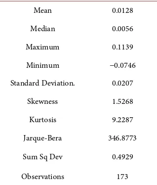
. The

(17)

DOI: 10.4236/am.2019.1012073 1064 Applied Mathematics [82]. For the period under analysis Table 1 shows that the mean, the maximum, and minimum inflation rates are 1.3, 11.4, −7.5 percentages respectively. (ii) With the Jarque-Bera statistic, 346.8773, it indicates that the inflation rate does not follow the normal distribution. It is well known that the fundamental task in many statistical analyses is to characterize the location and variability of a data set. A further characterization of the data includes skewness and kurtosis. The Skewness statistics is a measure of symmetry, or more precisely, the lack of symmetry. A distribution, or data set, is symmetric if it looks the same to the left and right of the center point. The Skewness of 1.52 indicates the moderate level.

In statistics, the Kurtosis is a measure of whether the data are heavy-tailed or light-tailed relative to a normal distribution. That is, data sets with high kurtosis tend to have heavy tails, or outliers. Data sets with low kurtosis tend to have light tails, or lack of outliers. Kurtosis statistics of the inflation rate 9.23 more large than 3, and Jarque-Bera statistics indicate that inflation rate does not follow the normal distribution. With high kurtosis statistic, 9.2287, there is an indication of inflation volatility.

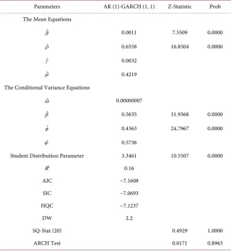
We use a Student statistic test of statistical significance and find that parame-ters estimations are all statistically significant. Results confirm that the past vola-tilities affect the current volatility of inflation rate. Thus, we the dynmical beha-vior of volatility. We restrict the constant term to a function of the GARCH pa-rameters and the unconditional variance:

1 2

1 1

ˆ 1 ,

q p

j i

w

σ

β

φ

−

= =

 

= _ − − _



∑



where 2 ˆ

σ _{is the unconditional variance of the residuals, that is,}

ω

ˆ=0.00000007. Table 2 raises tree isues. First, in the mean equation, the coefficient θ =ˆ1 0.6558

[image:17.595.293.452.530.717.2]

measuring the persistence of inflation rate is high. This means that the monthly last inflation contributes to current rate by 66 percents. Secondly, the stochastic

Table 1. Summary statistics.

Mean 0.0128

Median 0.0056

Maximum 0.1139

Minimum −0.0746

Standard Deviation. 0.0207

Skewness 1.5268

Kurtosis 9.2287

Jarque-Bera 346.8773 Sum Sq Dev 0.4929

(18)

[image:18.595.211.537.89.443.2]

Table 2. Results of estimation.

Parameters AR (1)-GARCH (1, 1) Z-Statistic Prob The Mean Equations

ˆ

ϑ 0.0011 7.5509 0.0000

ˆ

ρ 0.6558 16.8504 0.0000

ˆ

γ 0.0032

ˆ

µ 0.4219

The Conditional Variance Equations ˆ

ω 0.00000007

ˆ

β 0.5635 31.9568 0.0000

ˆ

φ 0.4363 24.7967 0.0000

ˆ

ψ 0.5736

Student Distribution Parameter 3.3461 10.5507 0.0000

R2 _0.16

AIC −7.1608

SIC −7.0693

HQC −7.1237

DW 2.2

SQ-Stat (20) 0.4929 1.0000

ARCH Test 0.0171 0.8963

volatility persistence of CPI-inflation rate is very high level,

0.5635 0.4363

+

=

0.9998

, this means that the past volatility information

con-tributes to current volatility of inflation rate at 100 percents. Therefore the pur-chasing power of congolese householders is also volatile.

The postestmation tests of Ljung Box (1978), Q-Stat = 3.0639, and ARCH test, 0.0171, show that there are any remaining ARCH effects in the residuals.

7. Concluding Remarks

(19)

Conflicts of Interest

The authors declare no conflicts of interest regarding the publication of this pa-per.

References

[1] Berg, T.O. (2017) Business Uncertainty and the Effectiveness of Fiscal Policy in Germany. MacroeconomicDynamics, 23, 1442-1470.

[2] Basu, S. and Bundick, B. (2017) Uncertainty Shocks in a Model of Effective De-mand. Econometrica, 85, 937-958.https://doi.org/10.3982/ECTA13960

[3] Basu, S. and Bundick, B. (2018) Uncertainty Shocks in a Model of Effective De-mand: Reply. Econometrica, 86.https://doi.org/10.2139/ssrn.3216683

[4] Kubzun, A.I. and Kan, Y.S. (1996) Stochastic Programming Problems with Proba-bility and Quantil Functions. John Wiley & Sons, New York.

[5] Möller, B. and Reuter, U. (2007) Uncertainty Forecasting in Engineering. Springer, New York.

[6] Sahalia, Y.A. (2002) Maximum Likelihood Estimation of Discretely Sampled Diffu-sions: A Closed-Form Approximation Approach. Econometrica, 70, 223-262.

https://doi.org/10.1111/1468-0262.00274

[7] Barndorff-Nielsen, O.E. and Shephard, N. (2004) Econometric Analysis of Realized Covariation: High Frequency Based Covariance, Regression, and Correlation in Fi-nancial Economics. Econometrica, 72, 885-925.

https://doi.org/10.1111/j.1468-0262.2004.00515.x

[8] Chernozhukov, V., Fernández-Val, I. and Luo, Y. (2018) The Sorted Effects Me-thod: Discovering Heterogeneous Effects beyond Their Averages. Econometrica, 86, 1911-1938. https://doi.org/10.3982/ECTA14415

[9] Hansen, L.P. (2012) Dynamic Valuation Decomposition within Stochastic Econo-mies. Econometrica, 80, 911-967.https://doi.org/10.3982/ECTA8070

[10] Hirano, K. and Wright, J.H. (2017) Forecasting with Model Uncertainty: Represen-tations and Risk Reduction. Econometrica, 85, 617-643.

https://doi.org/10.3982/ECTA13372

[11] Van Horne, J.C. and Wachowicz, J.M. (2008) Fundamentals of Financial Manage-ment. 13th Edition, Financial Times/Prentice Hall,Upper Saddle River, NJ.

[12] Stokey, N.L. (2009) The Economics of Inaction: Stochastic Control Models with Fixed Costs. Princeton University Press, Princeton, NJ.

https://doi.org/10.1515/9781400829811

[13] Francq, C. and Zakoian, J.M. (2010) GARCH Models Structure, Statistical inference and Financial Application. John Wiley and Sons, West Sussex.

https://doi.org/10.1002/9780470670057

[14] Lo, A.W. (1988) Maximum Likelihood Estimation of Generalized Itô Processes with Discretely Sampled Data. EconometricTheory, 4, 231-247.

https://doi.org/10.1017/S0266466600012044

[15] Prakasa Rao, B.L.S. (2010) Statistical Inference for Fractional Diffusion Processes. John Wiley and Sons, West Sussex.

[16] Ait Sahalia Y. and Jacod, J. (2014) High-Frequency Financial Econometrics. Prince-ton University Press, PrincePrince-ton, NJ.

https://doi.org/10.23943/princeton/9780691161433.001.0001