Interrogating the effect of an orifice on the upward two phase gas–liquid flow behavior

1

Interrogating the effect of an orifice on the upward two˗phase gas˗liquid flow behaviour

Ammar Zeghloula_{, Abdelwahid Azzi}a_{, Faiza Saidj}a_{, Barry J. Azzopardi}b_{, Buddhika}

Hewakandambyb

a _{University of Sciences and Technology Houari Boumedien (USTHB),}

FGMGP/LTPMP, Bab Ezzouar, 16111, Algiers, Algeria.

b _{Faculty of Engineering, University of Nottingham, University Park, NottinghamNG7}

2RD, United Kingdom.

Corresponding author: Abdelwahid AZZI, Tel: +213(0) 771 45 89 26, E˗mail: [email protected]

Abstract

2

Just downstream the orifice, the structure velocity increases for the bubbly and slug flows and decreases for churn flow. For bubble and slug flows, there is persistency of the frequency when passing through the orifice from the upstream to the downstream pipe.

Keywords:Orifice, two˗phase, upward, void fraction, conductance, frequency

Introduction

Gas˗liquid two˗phase flows through orifices are encountered in several industrial plants. Some examples are, flow characteristics of rupture discs, in engineering relief system of chemical reactors, leaks from ruptured vessels and pipes, in power generation units, control of two phase flow using choke valve on oil production platforms, desalination process by multistage flash (MSF) and the metering of two˗phase flows.

The evaluation of the pressure drop caused by the orifice and the knowledge of its upstream and downstream influences is necessary for safe and adequate design of the equipment where orifices might occur. There has been significant effort in modelling single˗phase flow through orifices and the corresponding pressure drops. Details of flow behaviour and models of pressure drops can be found in fluid mechanics textbooks such as Idel’chik (1994).

3

(2012) and to a lesser extent to the flow behaviour through orifices.

Fossa et al. (2006) investigated the slug pressure through sharp edge orifices in horizontal pipes. Time series of cross˗sectionally averaged void fraction were been measured using conductance probe technique upstream and downstream of the orifice which had dimensionless plate thickness of 0.023˗0.59 and area ratio of 0.54 and 0.73. They found that the void fraction usually reaches a maximum at a distance of about one diameter downstream of the throat. This maximum can be up to twice the value recorded in the fully developed flow regime far from the orifice. The flow in the developing region and the developing length (downstream the contraction) is also dependent on the upstream flow patterns and area ratio. Fossa and Guglielmini (2002) noticed that this behaviour was observed irrespective of the orifice thickness for high liquid flow rate and even more evident when the area ratio is low.

Recently Roul and Dash (2012) investigated numerically the behaviour of two˗phase air˗water flow through orifices placed in horizontal pipes. For their study, they used the same experimental conditions (flow conditions, orifice geometries) as those employed by of Fossa and Guglielmini (2002). They report finding similar to those of Fossa and Guglielmini.

Salcudean et al. (1983) analysed the effect of the flow obstructions on flow patterns and void fraction in horizontal tubes. They found that a central obstruction and an orifice plate influence on the flow pattern. The central obstruction was found to have the strongest effect on the transition between stratified smooth and stratified wavy and between stratified wavy and intermittent flows while the orifice plate has a stronger effect on the transition from intermittent to annular flow.

4

the narrowest flow cross˗section downstream the orifice divided by cross section of the pipe They worked with single phase and air˗water two phase flows in a horizontal pipe using a photographic technique. The results demonstrate that the contraction in the two˗phase flow is limited to very narrow ranges of mass flow qualities of less than 1.2 % and greater than 99 % where the flow regimes are bubbly and spray flow respectively.

Annular flow in vertical tube was studied by Azzopardi (1984) who examined the effect of thick orifices on the drop/film split. He used eight orifices with different angles of convergence/divergence, orifice diameter and thickness; he found that the film flow rates decreased after the contraction, subsequently returning back to the upstream value. He observed that the measured minimum film flow rate decreased with an increase in the angle and decrease in throat diameter. This work was extended by McQuillan and Whalley (1984) who presented similar results to those of Azzopardi (1984) from their study of effect of thin orifices on the film/drop split in annular flow. They noticed that the orifice plate caused extra atomisation of the film and the liquid returns to the film downstream the orifice plate.

For liquid-liquid mixture flow Chakrabarti et al. (2009) used the optical probe technique to analyse the influence of the orifice on the phase distribution during stratified water-kerosene flow. They concluded that this obstruction can be recommended as homogeniser/emulsifier for liquid-liquid systems. On the other hand from their study of pressure drop generated by this fitting they encouraged the use of the orifice as flow-metering device for liquid-liquid stratified flow.

5

They found that though the lengths of the Taylor bubbles and liquid slugs increase from upstream to downstream, the frequency essentially remains at the same value. They termed this persistence of frequency. They also found a similar behaviour between the pipe upstream and the throat of a Venturi and in pipeline˗bend˗riser arrangements in the work of , e.g., Saidj et al. (2014).

This paper is an attempt for understanding the fundamentals of the effect of the orifice on the two-phase flow behaviour through this fitting. It will be shown how the orifice geometry mainly affects bubbly, slug and churn flow patterns.The extent that this effect can persist downstream of the obstruction before the flow finally resumes the form that it has far upstream the orifice.

2. Experimental setup and the methodology

6

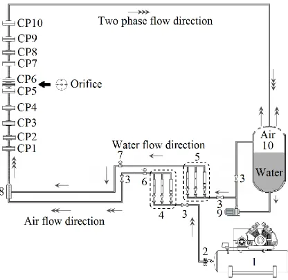
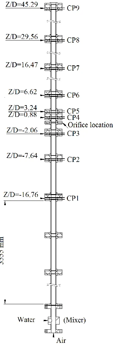
1: Compressor, 2: Pressure regulator, 3: Valve, 4: Air flowmeters, 5: Water flowmeters, 6: Manometer, 7: Thermometer, 8: Mixer, 9: Pump, 10: Tank/Separator, CP1˗CP9: Conductance probes

Fig. 1 Schematic diagram of the experimental facility

The vertical test section was made of transparent acrylic resin (PMMA), which permits visual observation of the flow pattern, is about 6m long with an inner diameter, Dt, of

7

The mixer made of Polyvinyl chloride (PVC) has a short concentric pipe, with 64 holes with 1 mm diameter spaced equally in 8 columns over a length of 80 mm on the cylindrical surface and with the top blanked off as the gas injector. The liquid is introduced into the annular chamber surrounding this gas injector , creating thus, a more even circumferential mixing effect.

Downstream the mixer, the air˗water mixture flows through the vertical pipe, a bend, a horizontal pipe and finally to the storage tank, where the air and the water are separated. The water is recirculated and the air is released to the atmosphere. Inflow of air and water are controlled by valve and metered using banks of calibrated rotameters mounted in parallel before the mixing unit. The maximum uncertainties in the liquid and gas flow rate measurements are 2%. The static pressure of the air flow is measured prior entering the mixing section. A thermometer with a precision of 0.1°C is used for temperature measurement. The temperature during the experiments was around 25°C. Tap water, which was used in the experiments, was found to have conductivity around 600 S/cm.

(measured with LUTRON YK-43C electrical conductivity meter). The electrical

conductivity showed an increasing with temperature. To avoid larges variations of

conductivity with the same experimental run, which could influence on the

measurement of the electrical resistivity of the medium, fresh water was fed

continuously to the storage tank and discharged to the drain.

A series of six orifices have been used in the present study. Table 1 summarizes the dimensions of these orifices. According to the criterion set by Chisholm (1983), orifices having t/Dt<0.5 can be classified as thin whilst those t/Dt>0.5 as thick.Thus, orifices 1,

8

Table1. Dimensions of the orifices

Orifice

Diameter, d

[mm]

Thickness, t

[mm]

Diameter ratio

σ=d/D

Thickness ratio

t/d

1 25 2.5 0.73 0.1

2 25 5 0.73 0.2

3 25 14.7 0.73 0.59

4 18.5 1.9 0.54 0.1

5 18.5 3.7 0.54 0.2

6 18.5 10.8 0.54 0.59

Since the water behaves as an electrical conducting medium and air as resistive medium, the conductance probe techniquehas been chosen to measure the void fraction. In this technique, the cross˗sectional averaged void fraction can be inferred once the relationship between electrical impedance and phase distribution has been established.

Fossa (1998), Abdulkadir et al. (2012), Saidj et al. (2014) are among other researchers who used this technique successfully.

9

10

The probes were constructed by mounting two stainless steel plates separated by a spacer between a pair of thick acrylic blocks and machining a hole through them so that they were flush with pipe inner wall. The configuration is characterised by the thickness of electrodes, s, and the distance between them, De.The dimensions De/Dt and s/Dtwere

0.264 and 0.058 respectively.

Measurements were made using an electronic circuit previously applied by Saidj et al. (2014) to measure void raction in gas liquid two phase flows. An excitation voltage of 1 V at 100kHz has been applied to this circuit. After elimination of the dc component, amplification, rectification and filtering, the signals are sent to data acquisition unit. The latter consists of a PC fitted with a Data acquisition Card (12 bits NI DAQ card˗6062E) employing LabView 8.6 software. Data were taken at a sampling frequency of 200 Hz over 60 seconds for each run.

In the present study, the probes have been excited using a signal with 0.1 MHz frequency, in such a way that the imaginary part of the impedance becomes negligible with respect to the real part. The impedance is therefore purely resistive.

The output voltage (Vout) given by the probe is proportional to the resistance of the

two˗phase mixture. This response is converted to dimensionless conductance (Ge*_{) by}

using the voltage obtained when the pipe is full of liquid (Vfull) as the reference value.

To account for the systemic errors, Vfull was measured before every experimental run

11 3. Results and discussion

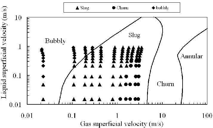
3.1 Flow pattern map

The gas and liquid superficial velocities studied ranged from 0.022 to 3.5 m/s and from

0.05 to 0.91 m/s respectively.

During a series of visual observations through the transparent vertical acrylic test

12

Fig. 3 Flow pattern map in the vertical pipe before the orifice

3.2 Void fraction time series before and after the orifice

13

flow both upstream and downstream the orifice. The void fractions are in proportion to their axial positions and individual slugs can be clearly traced.

Fig.4 Time series void fraction upstream and downstream orifice 1:Gas superficial velocity = 0.28 m/s, liquid superficial velocity = 0.3 m/s

3.3 PDFs of the void fraction time series before and after the orifice

14

15

Fig.5 Time series average void fraction upstream and downstream orifice 1:Gas superficial velocity = 0.28 m/s, liquid superficial velocity =0.3 m/s (orifice 1)

3.4 Spatial evolution of the average void fraction

The evolution of the average void fraction along the test section upstream and downstream the six orifices is plotted in Figure 6 for different gas and liquid superficial velocities combinations. For bubbly flow (Fig.6(a), (b)), the axial variation of the void fraction is different to what is seen for the slug and churn flow cases (Fig. 6(c) to Fig 6(d)).

16

as the post vena contracta velocity reduction. Further downstream the void fraction increases to reach a constant from the seventh probe (CP7) as the bubble size grow to a quasi stable distribution.

17

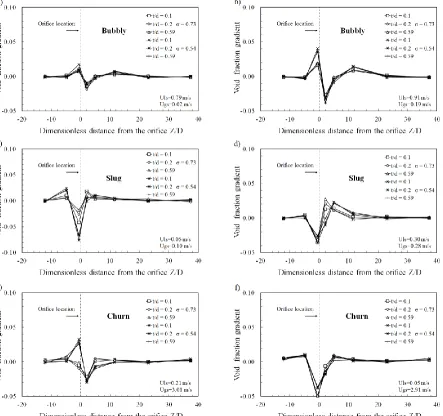
Fig.6 Evolution of the average void fraction along the test section upstream and downstream the orifices for different gas and liquid superficial velocities combinations 3-5 Spatial evolution of the void fraction gradients along the test section

18

increases before become 0 indicating constant void fraction at a distance of about 20 pipe diameter. Unlike bubbly flows, two intermittent flows (slug and churn), contrarily to bubbly flow, the gradient starts to decrease before the orifice, then increases through the orifice, decreases again and keeps a constant value at about 10D downstream the orifice for slug flow and about 7D for churn flow. For slug flow the effect of the orifice/pipe diameter area ratio on the void fraction is not high while for churn flow practically it does not exist.

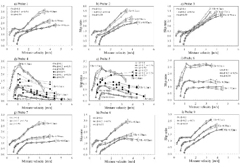
19 3.6 Slip ratio

In order to investigate the homogenization effect of the orifice on the two-phase flow, the slip ratio has been used. It is by definition the ratio of the mean gas velocity to that of the liquid phase,

S=UG UL

(1)

These velocities are related to the superficial velocities of the phases UGS and ULS and

the average void fraction, εG by:

U_G=UGS

ε_G 2 _and UL= U_LS

1 − 𝜀𝐺 3 The slip ratio reads:

S=UG U_L=

𝑈_𝐺𝑆 1-ε_G U_LSε_g (4)

In Figure 8(a) to 8(i), the evolution of the slip ratio as function of the mixture velocity (UM=ULS+UGS) along the test section, for orifices with low open are ratios (orifices 4, 5

and 6) is depicted. Equally, the experimental data obtained on slip ratios closely downstream the orifice by Fossa et al. (2006) during their experiments on the effect of orifices on horizontal intermittent flow are plotted in Figure 8(d) and 8(e). In Figure 8(d) the data of Fossa et al. are those obtained for orifice with the open area ratio equal to 0.54, at the distance Z/D between 0.3 and 0.7 downstream the orifice, and in Figure 8(e) between Z/D 1.9 and 2.3.

20

slip ratio curves are close each other despite the changing of the orifices’ thicknesses, implying that the thickness does not affect the slip ratio.

The influence of the liquid superficial velocity on the slip ratio is apparent. At low liquid superficial velocity ULS=0.3 m/s, the slip ratio can reach the value of about 3

while for higher velocities it decreases and can reach the value of less than one. This finding has been also reported by Fossa et al (2006).

At probe 4 (1D downstream the orifice), the whole values of the slip ratio are not equal to unity except for very few cases, which implies that at this position, the homogenization does not take place for these lower open area ratio orifices. The same observations could be made for the data of Fossa et al. These latter have been represented with filled symbols with dashed lines

However, at probe 5 (3 D downstream the orifice), for the liquid superficial velocity equal to 0.58 m/s, the whole values of the slip ratio lye around the unity, showing the homogenization effect of the orifice at this position. Further downstream, at probe 6 (at 7D downstream the orifice), we have also homogenization but for higher superficial liquid velocity, ULS=0.92 m/s. From this, one can conclude that the homogenization

21

Fig 8: Slip ratio as a function of the mixture velocity. Measuring location as parameter σ=0.54, Orifices 4, 5 and 6. Open symbols present study, Filled symbols Fossa et al. data

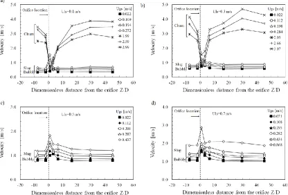
3.7 Spatial evolution of the structure velocity

The structure velocity along the test section are obtained by cross-correlating the void fraction times series between each successives paires of probes before and after the orifice.

22

At low liquid superficial velocity Fig 9(a), for both bubbly and slug flows, the structure velocity increases sharply just after the orifice, than decreases to finally stabilize at its initial value. However for the churn flow, the structure velocity decreases sharply when passing through the obstruction to lower velocities of less than 1 m/s. Same findings are obtained by increasing the liquid superficial velocity to 0.3 m/s (Fig 9 b). At high liquid superficial velocities, ULS equal to 0.7 m/s and 0.91 m/s Fig 9 (c) and 9 (d), the same

constatations could be reported on the evolution of the structure velocity when passing through the orifice.

Fig. 9 Evolution of the structure velocity along the test section for orifice 1.

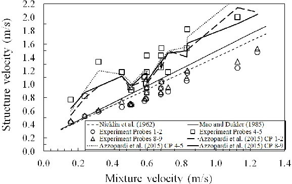
3.8 Structure velocity in Slug flow

In this section more attention is given to analyse the structure velocity within the slug

flow pattern. The values of the structure velocities obtained by cross-correlating the

23

chosen for orifice 1. The obtained experimental values of these velocities along with

those predicted by the correaltions of Nicklin et al. (1962), Mao and Dukler (1985) and

by Azzopardi et al .(2015) are plotted in figure 10.

Figure 10 shows that the values obtained far downstream and upstream the orifice are close together confirming the establishment and re-establishment of the flow at these distances. They are closer to the correlations of Nicklin et al. and that of Mao and Dukler but lower than those predicted by Azzopardi et al. The values computed immediately after the orifice are much higher than the two other ones. The structure velocity is increased about practically two times its initial values and is well predicted by the correlation of Azzopardi et al. An effect of the orifice is to move a small part of the gas in the Taylor bubble into the following liquid slug. Though this amount of gas makes little difference to the Taylor bubble, the increase in the void fraction in the liquid slug makes the following Taylor bubble more peaky and it will move faster as shown by Hills and Darton (1976), thus making the measured velocity higher.

24

3.9 Liquid film around the Taylor bubble for slug flow :

As one can expect, the Taylor bubble which covers most of the cross section area of the pipe, and which is surrounded by the liquid film, could be deformed or destroyed when passing through the orifice. As a consequence the film thickness could change and be used as a parameter to control the Taylor bubble form, destruction and re-formation downstream the orifice and thus the re-forming of the slug flow.

The liquid film around the Taylor bubble can be extracted from the local void fraction.

From figure 11, if one considers that the film is uniform without waves, the void

fraction in the taylor bybble, _TB is:

2 TB T TB TB D d A A        

 (5)

By taking

2 d D TB 

 (6)

The film thickness reads:





2

D _

   (7)

with δ, the liquid film thickness in mm, D and d_TB the diameter of the pipe and the

Taylor bubble respectively, and εTB the measured void fraction in the Taylor bubble

25 Fig.11 Slug unit

The evolution of dimensionless liquid film thickness calculated from equation (7) versus the distance from orifice 1 is given in Figure 12.

For the two superficial liquid velocities the increase of the gas superficial velocity results in the decrease of the liquid film thickness.

26

decreasing of the film thickness is apparent showing the reforming of the initial Taylor bubble which can be noticed from CP7 to CP9.

Fig.12 Liquid film thickness as a function of the distance from the orifice at liquid superficial velocity: (a) 0.05m/s, (b) 0.21m/s; (orifice 1)

3.10 Spatial evolution of the structure frequency

27

value from the upstream to the downstream pipe but with a slightly change just after the orifice due to the effect of this latter on this kind of flow pattern. Indeed the Taylor bubble after being disturbed by the orifice needs a certain distance to resume with its own frequency. For the lower liquid superficial velocity and higher gas velocities combinations, corresponding to churn flow pattern (Figure 13(c)), it appears clearly that the frequency does not show at all any persistency of the frequency. The frequency presents a random character along the test section.

In order to analyse the persistency caharacteristic for the whole combinations of gas and lquid superficial velocities for the studied orifices,1 to 6, the following criterion has been applied: there is persistency of frequency if (fi-f1)/f1 is less than 10%, with f1 the

frequency at the first probe, fi the frequency at the ith probe (i from 2 to 9). The analysis

of the whole data shows that there is persistency of the frequency through the orifice for the bubbly and slug flow and no persistensy for the churn flow.

28

The persistence of frequency found in the present results provides added support to the suggestion of universality across many fittings suggested by Azzopardi et al. (2014).

4. Conclusions

From the work presented above it can be concluded that:

 An orifice has an obvious effect on the gas/liquid flow passing through it. However, this effect is local and the flow quickly resumes the form it had upstream as it progresses along the downstream pipe.

 The recovery length for the return to the upstream condition is about 20, 10 and 7 pipe diameter downstream the orifice for the bubbly, slug and churn flow respectively.

 For homogenization of the flow, a minimum liquid superficial velocity is required. The position at which it occurs depends on the value of this velocity as well as on the fractional open area of the orifice.

 Just downstream the orifice, the structure velocity increases for the bubbly and slug flows and decreases for the churn flow and regain its initial value far downstream the obstruction.

 The values of the frequencies of periodic structures are very similar upstream and downstream the orifice for bubbly and slug flow indicating that there is persistence of frequency across this fitting similar to that reported by Azzopardi et al. (2014) for sudden contractions and pipeline˗bend˗riser arrangements.  The experiments presented here significantly extend the available data on the

29

previous work for this geometry has concentrated on annular flow by Azzopardi (1984), McQuillan and Whalley (1984).

References

Abdulkadir, M., Zhao, D., Azzi, A., Lowndes, I.S., Azzopardi, B.J., 2012. Two phase air˗water flow through a large diameter vertical 180° bend, Chem. Eng. Sci. 79, 138˗152.

Azzopardi, B.J., 1984. Annular two phase flow in constricted tubes. 1st National Heat Transfer Conference, Leeds, Institution of Chemical Engineers.

Azzopardi, B.J., Do, H.K., Azzi, A., Hernandez Perez, V., 2015. Characteristics of air/water flow in an intermediate diameter. Experimental Thermal and Fluid Science 60, 1˗8.

Azzopardi, B.J., Ijioma, A., Yang, S., Abdulkareem, L.A., Azzi, A., Abdulkadir, M., 2014. Persistence of frequency in gas˗liquid flows across a change in pipe diameter or orientation. International Journal of Multiphase Flow 67, supplement, 22-31.

Barnea, D., 1986. Transition from annular flow and from dispersed bubble flow˗Unified models for the whole range of pipe inclinations. International Journal of Multiphase Flow 12 (5), 733˗744.

Chakrabarti, D.P., Das, G., Das P.K., 2009. Liquid˗liquid two˗phase flow through an orifice. Chem. Eng. Comm. 196, 1117˗1129.

30

Costigan, G., Whalley, P.B., 1997. Slug flow regime identification from dynamic void fraction measurements in vertical air˗water flows. International Journal of Multiphase Flow 23, 263˗282.

Fitzsimmons, D.E., 1964. Two˗phasepressure drop in piping components. Report Hanford Laboratories HW˗80970, Rev. 1.

Fossa, M., 1998. Design and performance of a conductance probe for measuring liquid fraction in two˗phasegas˗liquid flow, J. of Flow Meas. and Inst. 9, 103–109.

Fossa, M., Guglielmini, G., 2002. Pressure drop and void fraction profiles during horizontal flow through thin and thick orifices, Experimental Thermal and Fluid Science 26 (5), 513–523.

Fossa, M., Guglielmini, G., Marchitto, A., 2006. Two˗phase flow structure close to orifice contractions during horizontal intermittent flows. International Communications in Heat and Mass Transfer 33, 698˗708.

Hills, J.H., Darton, R.C., 1976. Rising velocity of large bubble in a bubble swarm. Trans.I. Chem. Engrs. 54, 258-264.

Idel’chik, I.E., Malyavskayafs, G.R., Martynenko, O.G., Fried, E., 1994. Handbook of Hydraulic Resistances, 3rd edition, CRC Press.

Jayanti, S., Hewitt, G.F., 1992. Prediction of the slug˗to˗churn flow transition in vertical two˗phase flow. International Journal of Multiphase Flow 18 (6), 847˗860.

31

Mao, Z.S., Dukler, A.E., 1985. Brief communication: rise velocity of Taylor bubble in a train of such bubbles in a flowing liquid. Chem. Eng. Sci. 40, 2158-2160.

McQuillan, K.W., Whalley, P.B., 1984. The effect of orifices on the liquid distribution in annular two˗phase flow, International Journal of Multiphase Flow 10, 721˗731.

Morris, S.D., 1985.Two˗phase pressure drop across valves and orifice plates, European Two Phase Flow Group Meeting, Marchwood Engineering Laboratories, Southampton, UK.

Nicklin, D.J., Wilkes, J.O., Davidson, J.F., 1962. Two˗phase flow in vertical tubes, Trans. of Inst. of Chem. Eng. 40, 61˗68.

Roul, M.K., Dash, S.K., 2012. Numerical investigation of single and two˗phase flow through thin orifices in horizontal pipes. Indian Journal of Science and Technology 5 (9), 3274˗3280.

Roul, M.K., Dash, S.K., 2012. Single˗phase and two˗phase flow through thin and thick orifices in horizontal pipes. Journal of Fluids Engineering 134 1˗14.

Saadawi, A.A., Grattan, E., Dempster, W.M., 1999. Two˗phase pressure loss in orifice plates and gate valves in large diameter pipes, in: G.P. Celata, P. Di Marco, R.K. Shah (Eds.), 2nd Symp. Two˗Phase Flow Modelling and Experimentation, ETS, Pisa, Italy.

32

Salcudean, M., Chun, C.H., Groenveld, D.C., 1983. Effect of flow obstructions on void distribution in horizontal air˗water flow. International Journal of Multiphase Flow 9, 91˗96.

Shannak, B., Friedel, L., Alhusein, M., Azzi, A., 1999. Experimental investigation of contraction in single˗ and two˗phase flow through sharp˗edged short orifice. Forshungimingenieurwesen 64, 291˗295.

Shoham, O., 2006. Mechanistic modelling of Gas˗liquidtwo˗phase flow in pipes. Society of Petroleum Engineering, USA.

Simpson, H.C., Rooney, D.H., Grattan, E., 1983. Two˗phase flow through gate valves and orifice plates, Int. Conf. Physical Modelling of Multi˗Phase Flow, Coventry.