Generating uncountable transformation semigroups

(1)

SEMIGROUPS

Yann Péresse

A Thesis Submitted for the Degree of PhD at the

University of St. Andrews

2009

Full metadata for this item is available in the St Andrews Digital Research Repository

at:

https://research-repository.st-andrews.ac.uk/

Please use this identifier to cite or link to this item: http://hdl.handle.net/10023/867

(2)

Generating Uncountable Transformation

Semigroups

Yann P´eresse

(3)

been written by me, that it is the record of work carried out by me and that it has not been submitted in any previous application for a higher degree.

I was admitted as a research student in October 2005 and as a candidate for the degree of PhD in October 2005; the higher study for which this is a record was carried out in the University of St Andrews between 2005 and 2009.

Date 4/12/2009 Signature of candidate

I hereby certify that the candidate has fulfilled the conditions of the Resolution and Regulations appropriate for the degree of Ph.D. in the University of St Andrews and that the candidate is qualified to submit this thesis in application for that degree.

Date 4/12/2009

Signature of supervisor (Martyn Quick)

Signature of supervisor (James D. Mitchell)

In submitting this thesis to the University of St Andrews we understand that we are giving permission for it to be made available for use in accordance with the regulations of the University Library for the time being in force, subject to any copyright vested in the work not being affected thereby. We also understand that the title and the abstract will be published, and that a copy of the work may be made and supplied to any bona fide library or research worker, that my thesis will be electronically accessible for personal or research use unless exempt by award of an embargo as requested below, and that the library has the right to migrate my thesis

into new electronic forms as required to ensure continued access to the thesis. We have obtained any third-party copyright permissions that may be required in order to allow such access and migration, or have requested the appropriate embargo below.

The following is an agreed request by candidate and supervisor regarding the electronic publication of this thesis:

Access to Printed copy and electronic publication of thesis through the University of St Andrews.

Date 4/12/2009

Signature of candidate

Signature of supervisor (Martyn Quick)

(4)

Abstract

We consider naturally occurring, uncountable transformation semigroups S and in-vestigate the following three questions.

(i) Is every countable subsetF of S also a subset of a ﬁnitely generated subsemi-group of S? If so, what is the least number n such that for every countable subset F of S there exist n elements of S that generate a subsemigroup of S

containingF as a subset.

(ii) Given a subset U of S, what is the least cardinality of a subset A of S such that the union of A and U is a generating set forS?

(iii) Deﬁne a preorder relation4 on the subsets ofS as follows. For subsetsV and

W of S write V 4 W if there exists a countable subset C of S such that V

is contained in the semigroup generated by the union of W and C. Given a subset U of S, where does U lie in the preorder4 on subsets of S?

Semigroups S for which we answer question (i) include: the semigroups of the injec-tive functions and the surjecinjec-tive functions on a countably inﬁnite set; the semigroups

of the increasing functions, the Lebesgue measurable functions, and the diﬀerentiable

functions on the closed unit interval [0,1]; and the endomorphism semigroup of the random graph.

(5)

We investigate questions (ii) and (iii) in the case where S is the semigroup ΩΩ

of all functions on a countably inﬁnite set Ω. Subsets U of ΩΩ _{under consideration}

are semigroups of Lipschitz functions on Ω with respect to discrete metrics on Ω and

(6)

Thanks

To my supervisors and collaborators James Mitchell and Martyn Quick for the

knowl-edge, time and encouragements that I received from them.

To my other collaborators Micha l Morayne and Jacek Cicho´n for some enjoyable

and productive research meetings.

To Victor Maltcev for the long meetings and his inﬁnite enthusiasm for inﬁnite

semigroups.

To Nik Ruˇskuc, Robert Gray, Simon Craik and Max Neunh¨oﬀer for taking an

interest in my work and some very helpful mathematical discussions.

To Fiona Brunk, Hannah Coutts and Jonathan Bagnall for combining into, what

can be shown to be, the best possible mix of oﬃce mates.

To John MacQuarrie for proof-reading and other heroic acts.

To my family for supporting me even if some of them “do not believe in logic”.

To Graeme Kemp for housing me.

To my friends for patiently listening to what some consider conversation

incom-patible with social gatherings — such as the three door problem or lengthy

explana-tions of Cantor’s diagonalization process.

To Kirsty Alexander for not being put oﬀ by said explanations.

To anyone who reads this thesis.

(7)

(8)

Chapter 1 Introduction and background

1.1 Introduction

Functions are one of the most fundamental concepts within mathematics and the

study of diﬀerent aspects of functions pervades the subject. We will take an algebraic

outlook on functions and study their composition. In other words, we let Ω be a set

and study subsemigroups of the semigroup ΩΩ _{of all functions from Ω to Ω. Such}

semigroups are called transformation semigroups.

When presented with a semigroup, or any other algebraic structure for that

mat-ter, one of the ﬁrst things that any algebraist would like to know is how it is generated.

As usual, for a subset U of a semigroup S the subsemigroup generated by U, which we will denote by hU i, is the intersection of all subsemigroups of S containing U

as a subset. This is equivalent to saying that hU i consists of all ﬁnite products of elements of U. If hU i=S, then U is a generating set for S.

To have a generating set at hand can be very helpful when trying to deal with

the corresponding semigroup, especially when the generating set is small compared

(13)

to the semigroup itself. A small generating set oﬀers a succinct way of specifying the

semigroup as well as a tool to answer certain questions about it. An easy example of

the latter is the fact that a semigroup is commutative if and only if all its generators

commute.

Simply knowing whether a given semigroup has a small generating set can give

some idea about the structure and complexity of the semigroup. For example, if

one was asked for the key diﬀerence between the semigroups of the natural numbers

N = {1,2,3, . . .} under addition and N under multiplication, one would probably

point to the fact, that N under addition is generated by the element 1, whereas N

under multiplication is not generated by any ﬁnite subset of N.

It is therefore very natural to ask for the smallest cardinality of a generating set

for a given semigroup. This smallest cardinality is usually called the rank of the semigroup.

In this thesis we are interested in subsemigroups of ΩΩ _{for inﬁnite sets Ω. This}

means that most of the semigroups under consideration will be uncountable. Of

course, an uncountable semigroupScannot have ﬁnite rank, since any ﬁnite subset of

S generates an at most countably inﬁnite subsemigroup ofS. In fact, the question of the rank of S becomes entirely trivial whenS is an uncountable semigroup. Suppose that an inﬁnite subset G of S generates S. Then

S =G1∪G2 ∪G3∪. . . where Gn={g1g2· · ·gn : g1, g2, . . . , gn∈G}.

But |Gn_| ₌ _|G| _{for any} _n _∈ _N _{and so} _|S| ₆ P∞

n=1|G

n_| ₌ _|G|_{. So the rank of any}

uncountable semigroup S is just|S|.

A remark about set theory: the above argument implicitly uses the Axiom of

Choice (see Section 2.3 for more details). In fact, most of the results presented in

(14)

1.2. SIERPI ´NSKI RANK 13

axiom. We will continue to use the Axiom of Choice without apology or explicit

reference.

Since, for uncountable semigroups, the usual endeavour of ﬁnding generating

sets of small cardinality is futile and the question of rank trivial, mathematicians

have introduced several alternative generation properties that do make sense for

uncountable semigroups. In this thesis we will study the following three ideas.

Firstly, instead of trying to generate the entire uncountable semigroupS, we could ask for the smallest number of elements of S needed to generate a subsemigroup containing any given countable subset of S. Another idea is to assume that we ‘already have’ a large subset U of S and to try and ﬁnd the smallest set A⊆S such that U ∪A generates S (see Section 1.3 for a precise formulation). The ﬁnal notion is to, in some sense, order the subsets of S according to their generating strength.

We will now introduce these three ideas in detail and point out the connections

between them. Some background deﬁnitions, conventions and results that we will

use in this and later chapters may be found in Chapter 2.

1.2 Sierpi´

nski rank

A semigroup S has Sierpi´nski rank n if n is the least number such that for every countable subset F of S there exist g1, . . . , gn∈S such thatF ⊆ hg1, . . . , gni. If no

such n exists, then we will say that S has infinite Sierpi´nski rank.

The reason for this name and the starting point for this section is the following

theorem by Sierpi´nski [29] from 1935.

Theorem 1.2.1. Let Ω be an infinite set and let f1, f2, . . .∈ΩΩ be arbitrary. Then

(15)

The proof included here is due to Banach [3] and much shorter than Sierpi´nski’s

original proof. The proof uses the notion of a moiety that will be important

through-out the thesis. Amoiety of an inﬁnite set Ω is a subset Λ⊆Ω such that|Λ|=|Ω\Λ|=

|Ω|.

Proof of Theorem 1.2.1. Partition the set Ω into countably many moieties Ω0,Ω1,Ω2, . . .

and partition Ω0 into countably many moieties

Ω0,1,Ω0,2,Ω0,3, . . . .

Let g ∈ΩΩ _{be any function that maps Ω}

i−1 bijectively to Ωi for all i∈N.

We will now deﬁneh ∈ΩΩ _{in two steps. Let} _h _{map Ω}

i bijectively to Ω0,i for all

i ∈ N. Note that, so far, h is only deﬁned on Ω\Ω0. Nevertheless, for any i ∈ N,

the composite function

ti =ghgih: Ω−→Ω0,i

is already deﬁned and ti is a bijection from Ω to Ω0,i. Now deﬁneh on Ω0 by

αh =αt−_i 1fi for all α∈Ω0,i and for alli∈N.

We will now show that every fi satisﬁes fi =ghgih2. Let α ∈ Ω be arbitrary, then

αghgi_h₌_αt

i ∈Ω0,i and so

αghgih2 =αtih=αtit−i 1fi =αfi.

Hence {f1, f2, . . .} ⊆ hg, hi as required.

Another way of stating Theorem 1.2.1 is to say that the Sierpi´nski rank of ΩΩ

(16)

1.2. SIERPI ´NSKI RANK 15

thought tells us that the answer is ‘no’: if a semigroupS has Sierpiński rank 1, then every countable subset of S is contained in a one-generator subsemigroup of S. In particular,Sis commutative. None of the semigroups that we will study with respect to Sierpiński rank are commutative, and so all Sierpiński ranks will be at least 2.

Banach’s proof above can be very easily adapted to obtain analogous results for

other semigroups. For example, the following was pointed out in [16]. Let f1, f2, . . .

in the proof of Theorem 1.2.1 be arbitrary partial maps on Ω or arbitrary binary

relations on Ω, instead of arbitrary functions on Ω. Then the very same argument

shows, respectively, that the semigroups of all partial maps on Ω and the semigroup

of all binary relations on Ω (under composition of binary relations) have Sierpi´nski

rank 2.

Upon seeing Theorem 1.2.1, the perhaps most natural question is to ask for the

Sierpi´nski rank of the symmetric group Sym(Ω). As usual, if G is a group and U is a subset of G, then the subgroup generated by U is the intersection of all subgroups of G that contain U as a subset. This is equivalent to saying that the subgroup generated by U is the set of all ﬁnite products of elements of U and their inverses.

It would be possible to define Sierpiński rank differently for groups so that it

would be in terms of generation of groups rather than semigroups. This is not the

approach we will take here. We will consider groups to simply be particular (and

particularly nice) examples of semigroups. In particular, even if U is a subset of a group, the notation hU i refers to the subsemigroup generated by U while the subgroup generated by U is hU, U−1 _i _where _U−1 ₌ _{_u−1 _: _u _∈ _U _} _{is the set of}

inverses of elements of U.

F. Galvin proved the following result.

(17)

subset F of Sym(Ω) there exists a subgroup G of Sym(Ω) generated by two elements of Sym(Ω) such that F ⊆G.

Note that by our previous discussion, Theorem 1.2.2 does not imply that the

Sierpi´nski rank of Sym(Ω) is 2 but merely that it is at most 4. However, Galvin also

considered the problem of restricting the orders of the generators.

Theorem 1.2.3. [13, Theorem 3.5] Let Ω be an infinite set. For every countable subset F of Sym(Ω) there exists a subgroup G of Sym(Ω) generated by two elements of Sym(Ω), one of order 53 and the other of order 4, such that F ⊆G.

Theorem 1.2.3 immediately implies the precise value of the Sierpi´nski rank of

Sym(Ω).

Theorem 1.2.4. Let Ωbe an infinite set. Then the Sierpi´nski rank of Sym(Ω) is 2. Proof. Let F be a countable subset of Sym(Ω). By Theorem 1.2.3 there existf, g ∈

Sym(Ω) with ﬁnite orders such that F ⊆ hf, g, f−1_{, g}−1_i_{. Since} _f _and _g _{have ﬁnite}

orders it follows that f−1_{, g}−1 _{∈ h}_{f, g}_i _{and so} _h_{f, g}_i₌_h_{f, g, f}−1_{, g}−1_{i ⊇}_F_.

The Sierpi´nski ranks of some more semigroups are known. For example, Sierpi´nski

himself [28] proved1 _{that the Sierpi´}_{nski rank of the semigroup of continuous functions}

on the closed unit interval is at most 4. (Of course he did not use the term ‘Sierpi´nski

rank’.) We will give his proof in Section 3.4 (see Lemma 3.4.2).

1_{Historically, this result actually precedes Sierpi´}_{nski’s other result (Theorem 1.2.1) by about a}

year. Theorem 1.2.1 is arguably better known and a more natural first result in this area and thus

was chosen as the motivation for the definition of Sierpi´nski rank. This can be seen as an example

of ‘history as it should have happened vs history as it really was’, a concept put forward by L. Olsen

in a lecture on complex numbers. According to Olsen, complex numbers arose from attempts to

(18)

1.3. RELATIVE RANK 17

The result was subsequently improved and generalised. S. Subbiah [30] showed

that the Sierpi´nski rank of the semigroup of continuous functions on certain

topo-logical spaces is 2. Topotopo-logical spaces where this result applies include [0,1]n_{for any}

n, the set of rational numbers and the set of irrational numbers.

K. D. Magill Jr. [23] showed that the semigroup of endomorphisms of an inﬁnite

dimensional vector space over a finite field has Sierpiński rank 2. This result has

been generalised in [2] where it was shown that the semigroup of endomorphisms of

any algebra with inﬁnite independent generating set has Sierpi´nski rank 2.

In Chapter 3 we will calculate the Sierpi´nski rank for several naturally occurring

transformation semigroups. (See Section 3.1 for an overview of the results in Chapter

3.)

1.3 Relative rank

Let S be a semigroup and let U be a subset of S. The relative rank ofS modulo U, denoted by rank(S : U), is deﬁned to be the least cardinality of a set A ⊆ S such that hU, Ai=S. We may also call rank(S :U) the relative rank of U in S.

Relative ranks of transformation semigroups were ﬁrst explicitly considered in

[20] and [21]. In the latter it was shown that if Ω is any inﬁnite set, then rank(ΩΩ _:

Sym(Ω)) = 2 and rank(ΩΩ _:_E_{(Ω)) = 2, where} _E_{(Ω) is the set of idempotents of Ω}Ω_.

As usual, an idempotent of a semigroup S is an element e of S such that e2 ₌ _e_.

The pairs of elements of ΩΩ _{that generate Ω}Ω _{together with Sym(Ω) and the pairs}

of elements of ΩΩ _{that generate Ω}Ω _{together with} _E_{(Ω) were also classiﬁed in [21].}

Before we give proofs of the facts that rank(ΩΩ _{: Sym(Ω)) = 2 and rank(Ω}Ω _:

E(Ω)) = 2 here, we will point out some connections between the notions of relative

(19)

The group cofinality of a non-finitely generated group G is the minimal length of an infinite chain of proper subgroups of G whose union is G. The semigroup cofinality of a non-finitely generated semigroup S is analogously defined to be the minimal length of an infinite chain of proper subsemigroups of S whose union is S. For a non-finitely generated groupG, the group cofinality ofG equals the semigroup cofinality of G (see [24, Lemma 2.1]). We denote the semigroup cofinality of S by cf(S).

Theorem 1.3.1. [22, Theorem 1.1.] Let Ω be an infinite set. Then cf(Sym(Ω)) > |Ω|.

The proof of [22, Theorem 1.1] can be adapted to obtain the analogue for ΩΩ_.

For a proof see [25, Proposition 4].

Theorem 1.3.2. Let Ω be an infinite set. Then cf(ΩΩ₎_>_|_Ω_|_.

The relative ranks that a semigroup S may have modulo any of its subsets are restricted by the Sierpi´nski rank of S and cf(S). Denote the least uncountable cardinal by ℵ1.

Proposition 1.3.3. Let S be a semigroup with Sierpiński rank n ∈N and let U be a subset of S. Then either rank(S:U)6n or rank(S:U)>max{cf(S),ℵ1}. Proof. First, suppose that rank(S : U) 6 ℵ0. Then, by definition, there exists a countable subset F of S such thathU, F i=S. Since the Sierpiński rank of S isn, there exist g1, . . . , gn ∈ S such that F ⊆ hg1, . . . , gni. Hence hU, g1, . . . , gni = S

and so rank(S :U)6n.

Now suppose that rank(S : U) > ℵ1. Let κ be the least ordinal of cardinality

(20)

Let A = {aλ}λ<κ be a subset of S such that hU, Ai = S. Then for any µ < κ

the semigroup Sµ = h {aλ}λ<µ, U i is a proper subsemigroup of S. Furthermore,

Sµ ⊆ Sν whenever µ 6 ν. It follows that {Sµ}µ<κ is a chain of length κ of proper

subsemigroups of S whose union is S and hence κ>cf(S).

For ΩΩ _{and Sym(Ω) we obtain the following corollaries of Proposition 1.3.3 and}

Theorems 1.2.1, 1.2.4, 1.3.1 and 1.3.2.

Corollary 1.3.4. Let Ω be an infinite set and let U be a subset of ΩΩ_{. Then either}

rank(ΩΩ _:_U₎₆₂ _or _rank(ΩΩ _:_U₎_>_|_Ω_|_.

Corollary 1.3.5. Let Ω be an infinite set and let U be a subset of Sym(Ω). Then either rank(Sym(Ω) :U)62 or rank(Sym(Ω) :U)>|Ω|.

The following is another theorem due to Galvin.

Theorem 1.3.6. [13, Theorem 5.8] Let Ωbe an infinite set and let q>2be a natural number. Let AandB be subsets ofSym(Ω) such that the group generated byA∪B is

Sym(Ω). If |B|6|Ω|, then there exists g ∈Sym(Ω) of order 2q such that the group generated by A∪ {g} is Sym(Ω).

For subgroupsG of Sym(Ω) it is possible to restrict the values of rank(Sym(Ω) :

G) even further.

Corollary 1.3.7. Let Ω be an infinite set and letU be a subset of Sym(Ω) such that

U−1 ₌_U_{. Then either} _{rank(Sym(Ω) :}_U₎₆₁ _or _{rank(Sym(Ω) :}_U₎_>_|_Ω_|_.

Proof. If rank(Sym(Ω) :U)6|Ω|, then, by deﬁnition, there existsB ⊆Sym(Ω) with

|B| 6 |Ω| and hU, B i = Sym(Ω). In particular, the group generated by U ∪B is Sym(Ω) and so by Theorem 1.3.6 there existsg ∈Sym(Ω) with ﬁnite order such that the group generated by U ∪ {g}is Sym(Ω). Since U−1 _⊆_U _and _g _{has ﬁnite order it}

(21)

Provided that we know the Sierpi´nski rank of a semigroup S, Proposition 1.3.3 gives us restrictions on the possible values of the relative ranks of S modulo its subsets. The next theorem, which will be used in Chapter 3, provides an upper

bound for the Sierpi´nski rank of S provided that we know the relative rank and the Sierpi´nski rank of one of its subsemigroups.

Theorem 1.3.8. Let S be a semigroup and let T be a subsemigroup of S. Suppose

rank(S : T) = m and the Sierpi´nski rank of T is n for some m, n ∈ N. Then the Sierpi´nski rank of S is at most m+n.

Proof. There exists1, s2, . . . , sm ∈S such thaths1, s2, . . . , sm, Ti=S. Letf1, f2, . . .

be arbitrary elements of S. For each fi there exists a ﬁnite set Gi ⊆ T such that

fi ∈ hs1, s2, . . . , sm, Gii. SinceG=Si∈NGi is countable there existg1, g2, . . . , gn∈T such that G⊆ hg1, g2, . . . , gni. Thus

{f1, f2, . . .} ⊆ hs1, s2, . . . , sm, Gi ⊆ hs1, s2, . . . , sm, g1, g2, . . . , gni

which concludes the proof.

In this thesis we are particularly interested in relative ranks of ΩΩ _{modulo its}

subsets. Given the split between “very ﬁnite” and “very inﬁnite” relative ranks in

ΩΩ _{(see Corollary 1.3.4) we would like to have some method of telling whether or not}

a given subset U of ΩΩ _{has ﬁnite relative rank in Ω}Ω_{. The following is a suﬃcient}

condition.

Lemma 1.3.9. Let Ω be an infinite set and let U ⊆ΩΩ_{. If there exists} _Λ _⊆_Ω _with |Λ| =|Ω| and non-empty, pairwise disjoint subsets (Ωω)ω∈Ω of Ω such that, for any

map t∗ _{: Λ}_{−→ {}_Ω

ω : ω ∈Ω}, there exists t ∈ hUisuch that λt∈λt∗ for all λ∈Λ,

(22)

Proof. Let g be a bijection from Ω to Λ. Then g ∈ ΩΩ_{. Let} _h _∈ _ΩΩ _{be deﬁned by} αh =ω for all α∈Ωω for all ω∈Ω. We will show that ΩΩ =hU, g, hi.

Letf ∈ΩΩ _{be arbitrary. Let}_t∗ _{: Λ}_{−→ {}_Ω

ω : ω ∈Ω}be deﬁned byλt∗ = Ωλg−1_f

for all λ ∈ Λ. By assumption, there exists t ∈ hU i such that λt ∈ Ωλg−1_f for all

λ∈Λ.

Now ifα is any element of Ω, thenαg∈Λ and so (αg)t∈Ω(αg)g−1_f = Ω_αf. Hence

αgth=αf. Thus gth=f and hU, g, hi= ΩΩ_{, since} _f _{was arbitrary.}

It is not known whether there exist any subsets U of ΩΩ _{with ﬁnite relative rank}

in ΩΩ _{that do not fulﬁl the condition of Lemma 1.3.9. In particular, we will see that}

the lemma allows us to show that rank(ΩΩ _{: Sym(Ω))}₆_{2 and rank(Ω}Ω _:_E_(Ω))₆_2.

To obtain lower bounds for relative ranks of subsets of ΩΩ_{, we require the following}

lemma, which will be used again in Chapter 6.

Lemma 1.3.10. Let U be a subset of ΩΩ _{such that} _f _∈_U _{is injective if and only if} f is surjective. Then rank(ΩΩ _:_U₎_>₂_.

Proof. Seeking a contradiction assume that hU, g i = ΩΩ _{for some} _g _∈ _ΩΩ_{. Let} h∈ΩΩ _{be injective but not surjective and let}_k _∈_ΩΩ _{be surjective but not injective.}

Then there exist h1, h2, . . . , hm, k1, k2, . . . , kn ∈ U ∪ {g} such that h = h1h2· · ·hm

and k =k1k2· · ·kn.

Let

M = min{i : h1h2· · ·hi is not surjective}

and

N = max{i : kiki+1· · ·kn is not injective}.

Since h is injective, h1· · ·hM is injective but not surjective. Similarly, since k is

surjective, kN· · ·kn is surjective but not injective. We will now show that hM is

(23)

If M = 1, then hM = h1· · ·hM is injective but not surjective. If M > 1, then

by deﬁnition of M, the function h1· · ·hM−1 is surjective. Since h1· · ·hM−1hM is

injective it follows that h1· · ·hM−1 is also injective and hence bijective. HencehM is

injective but not surjective, since h1· · ·hM−1hM is injective but not surjective. Thus

hM =g.

Similarly, ifN =n, thenkN =kN· · ·kn is surjective but not injective. If N < n,

then kN+1· · ·kn is injective by deﬁnition of N. Since kNkN+1· · ·kn is surjective it

follows that kN+1· · ·kn is surjective and hence bijective. Thus kN is surjective but

not injective since kNkN+1. . . kn is surjective but not injective. Hence kN = g, a

contradiction since kN 6=hM.

Theorem 1.3.11. [21, Theorem 3.3] Let Ω be an infinite set. Then rank(ΩΩ _:

Sym(Ω)) = 2.

Proof. To show that rank(ΩΩ _{: Sym(Ω))} ₆ _{2, let Λ be any moiety of Ω and let}

(Ωω)ω∈Ω be disjoint moieties of Λ. Let t∗ be any map from Λ to {Ωω : ω ∈Ω}.

Let k : Λ −→ Ω be any injection such that λk ∈ λt∗ _{for all} _λ _∈ _{Λ. Such an} injective k exists, because |Ωω| =|Λ| for every ω ∈ Ω. Now since k is injective and

|Ω\dom(k)|=|Ω\im(k)|we may extend k to an elementt of Sym(Ω). By Lemma 1.3.9 it follows that rank(ΩΩ_{: Sym(Ω))}₆_2.

On the other hand rank(ΩΩ _{: Sym(Ω))} _> _{2 by Lemma 1.3.10 since every} _f _∈

Sym(Ω) is both injective and surjective.

Theorem 1.3.12. [21, Theorem 5.1] Let Ω be an infinite set. Then rank(ΩΩ _: E(Ω)) = 2.

Proof. Recall that an element of ΩΩ _{is an idempotent if and only if it is the identity}

(24)

of Ω. Let t∗ _{be any function from Λ to the set of singletons} _{{ {σ}} _: _σ _∈ _Σ_}_{. Let}

t∈ΩΩ _{be deﬁned by}

αt=

    

σ if α ∈Λ with αt∗ ₌_{σ}

α if α ∈Ω\Λ.

Since Λ and Σ are disjoint, im(t) = Ω\Λ and so tis the identity on its image. Hence

t is an idempotent and so it follows by Lemma 1.3.9 that rank(ΩΩ _:_E_(Ω))₆_2.

On the other hand, rank(ΩΩ _:_E_(Ω))_>_{2 by Lemma 1.3.10 since the only injective} f ∈ E(Ω) is the identity.

Theorems 1.3.11 and 1.3.12 have subsequently, in [1], been generalised into the

context of endomorphisms of independence algebras which are essentially

generali-sations of vector spaces in the context of universal algebra.

Another class of subsets of ΩΩ _{for which the relative ranks in Ω}Ω _{have been}

investigated are endomorphisms of partial orders on Ω. In [16] it was shown that

the order endomorphisms of the natural numbers Nhave relative rank 1 in NN . This

result has been generalised in two diﬀerent ways.

In [18] it was shown that if Ω is a countable totally ordered set or a well ordered

set of arbitrary cardinality, then the order endomorphisms of Ω have relative rank 1

in ΩΩ_.

Countable partially ordered sets (Ω,⊑) were considered in [17]. It was shown that if (Ω,⊑) has inﬁnitely many connected components, then the rank of the order endomorphisms End(Ω,⊑) of (Ω,⊑) in ΩΩ _{is 1. On the other hand, if (Ω}_,_⊑_{) has}

ﬁnitely many connected components, then rank(ΩΩ _{: End(Ω}_,_⊑_{)) is ﬁnite, and hence}

at most 2, if and only if there are inﬁnitely manyα∈Ω for which {β ∈Ω : α⊑β}

(25)

End(Ω,⊑)) = 2 was also constructed in [17]. We will extend some of the results from [17] in Chapter 6.

The methods used in [17] to prove that rank(ΩΩ _{: End(Ω}_,_⊑_{)) is uncountable}

under the appropriate conditions on (Ω,⊑), led to the investigation in [10] of the relative ranks of semigroups of continuous functions on a metric space Ω modulo the

set of Lipschitz functions on Ω. It was shown that this rank is uncountable for a

wide class of metric spaces Ω. Examples of metric spaces included in this class are

the natural numbersN, the integersZ, the rational numbersQand the real numbers

R under the usual Euclidean metric. Also included are all metric spaces that arise

from connected locally ﬁnite graphs with countable vertex set Ω, where the distance

between two vertices is the minimal length of a path between them.

Note that in the case when Ω is derived from a graph, the metric on Ω is

dis-crete and so the semigroup of continuous functions is just ΩΩ_{. Furthermore, every}

endomorphism of the graph is a Lipschitz function on Ω and so the results from [17]

imply that the endomorphisms of a connected locally ﬁnite graph with countable

vertex set Ω have uncountable relative rank in ΩΩ_{. This line of research will also be}

continued in Chapter 6.

The Baire space N is the topological space of all sequences of natural numbers

under the topology of pointwise convergence (see Section 2.5). Another interesting

result from [10] is that the relative rank of the semigroup of continuous functions on

N modulo the Lipschitz functions on N is ℵ1. This is one of the ﬁrst non-trivial

examples where the exact value of an uncountable relative rank could be speciﬁed.

We will obtain similar results in Chapters 4, 5 and 6. More precisely, we will let

Ω be a countably inﬁnite set and specify the precise value of rank(ΩΩ _:_U_{) for several}

subsets U of ΩΩ _{that have uncountable relative rank in Ω}Ω_.

(26)

1.4. THE BERGMAN-SHELAH PREORDER 25

we assume the Continuum Hypothesis, then this task becomes trivial: ifU is a subset of ΩΩ_{which does not have ﬁnite relative rank in Ω}Ω_{, then}_ℵ

0 <rank(ΩΩ :U)62ℵ0 by

Corollary 1.3.4 and so, by the Continuum Hypothesis, rank(ΩΩ _:_U_{) = 2}ℵ0. However,

we will not assume the Continuum Hypothesis and, when given a subset U of ΩΩ_,

we will investigate the question of the precise value of rank(ΩΩ _: _U_{). The cardinal}

number d will be prominent and is described as follows.

Let Ω = {α1, α2, . . .}. Order Ω by αi 6 αj whenever i 6 j. (Alternatively,

assume that Ω = N.) A function f ∈ ΩΩ _{is said to} _dominate _{another function} g ∈ ΩΩ _if _αf _> _αg _{for all} _α _∈ _{Ω. A subset} _U _{of Ω}Ω _{dominates a family} _V _⊆ _ΩΩ _if

for all g ∈V there exists f ∈U such thatf dominates g. It was shown in [16] that if U is dominated by a countable subset of ΩΩ_{, then rank(Ω}Ω _:_U_{) is uncountable.}

The cardinal d _{is deﬁned to be the least cardinality of a subset of Ω}Ω _that

domi-nates ΩΩ_{. The following relations are not hard to obtain:} _ℵ0 _<_d₆₂ℵ0. (For a proof

see [17, Lemma 3.5]). It is consistent with the usual axioms of set theory (ZFC) that

d=ℵ1 <2ℵ0 =ℵ2 or ℵ1 <_d= 2ℵ0 =ℵ2, see [4].

In Chapter 4 we will show that if U is dominated by a countable subset of ΩΩ_,

then rank(ΩΩ _:_U₎_>_d_{. In Chapters 5 and 6 we will show that rank(Ω}Ω _:_T_{) =}_d _for

several naturally occurring subsemigroups T of ΩΩ_.

1.4 The Bergman-Shelah preorder

Throughout this section let Ω be a countably inﬁnite set. If G is any subgroup of Sym(Ω), then rank(Sym(Ω) : G) is either 1 or uncountable (see Corollary 1.3.7). Motivated by this “wide gap”, Bergman and Shelah [5] introduced the following order

relation which, in some sense, orders subsets of Sym(Ω) according to their generating

(27)

IfGandHare subsets of Sym(Ω), then we writeG4H if there exists a countable subset F of Sym(Ω) such that G is contained in the subgroup generated by H∪F.

Clearly G 4 G and if G4 H and H 4 K, then G 4 K for all G, H, K ⊆ Sym(Ω)

and so 4 is a preorder on the set of subsets of Sym(Ω).

Note that, by Galvin’s result (Theorem 1.2.4), the countable set F is contained in a ﬁnitely generated subgroup of Sym(Ω) and so the deﬁnition of 4 is equivalent to saying that G4H if there exists a finite (or evenof size at most 2) subset F of Sym(Ω) such that Gis contained in the subgroup generated by H∪F.

Like every preorder, 4 gives rise to an equivalence relation. Write G ≈ H to denote that G4H and H 4G. Then≈ is an equivalence relation on the subsets of Sym(Ω). We will write G≺H to denote that G4H and H64G.

There is a natural topology on Sym(Ω) — the topology of pointwise convergence

(or product topology). More information on the topology on Sym(Ω) can be found

in Section 2.5. Bergman and Shelah considered subgroups of Sym(Ω) that are closed

in the topology of pointwise convergence on Sym(Ω) and completely classiﬁed such

closed subgroups according to ≈.

One of the reasons that the class of closed subgroups of Sym(Ω) is of interest is

that it coincides with the automorphism groups of relational structures on Ω. An

n-ary relation on Ω is a set of n-tuples of elements of Ω. A relational structure on Ω is a set of relations on Ω. An endomorphism of a relational structure S on Ω is a function f ∈ ΩΩ _{such that for every relation} _R _∈ _S _{we have that (}_{β1, . . . , β}

n) ∈ R

implies that (β1f, . . . , βnf)∈R. Anautomorphism ofS is a bijective endomorphism

whose inverse is an endomorphism.

It is known and not diﬃcult to show that a subgroup of Sym(Ω) is closed if and

only if it is the automorphism group of a relational structure on Ω. Indeed, any

(28)

1.4. THE BERGMAN-SHELAH PREORDER 27

structure consisting of all relations of the form {(β1f, . . . , βnf) : f ∈ G} for some

β1, . . . , βn ∈ Ω. Similarly, a subsemigroup of ΩΩ is closed if and only if it is the

endomorphism semigroup of a relational structure on Ω (see [9, Section 6]).

The classiﬁcation in [5] of the closed subgroups of Sym(Ω) can be summarised

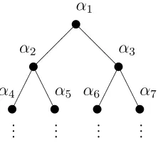
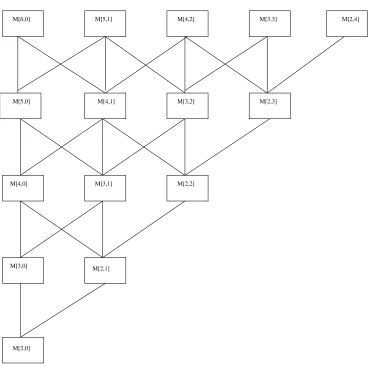
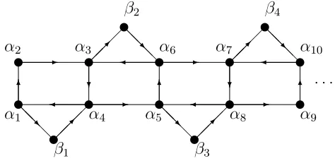
as follows. Let Ω = {α1, α2, . . .} and partition Ω into the sets Ai ={α2i−1, α2i} for

i ∈ N. Then let GA be the subgroup of Sym(Ω) consisting of all f ∈ Sym(Ω) such

that Aif =Ai for all i∈N. Similarly, partition Ω into the sets

B1 ={α1}, B2 ={α2, α3}, B3 ={α4, α5, α6}, B4 ={α7, α8, α9, α10}, . . .

and let GB be the subgroup of Sym(Ω) consisting of all f ∈ Sym(Ω) such that

Bif =Bi for alli∈N. Denote by 1Ω the identity function on Ω. It was shown in [5]

that

{1Ω} ≺GA≺GB ≺Sym(Ω). (1.1)

Furthermore, every closed subgroup G of Sym(Ω) is equivalent under ≈ to one of the groups in (1.1) above. Which of these subgroups G is equivalent to depends on the pointwise stabilisers G(Σ) ={g ∈G : αg =α for all α∈Σ}of ﬁnite subsets Σ

of Ω. As usual, for a subgroup G of Sym(Ω) and α ∈ Ω the set {αg : g ∈ G} is called an orbit of G.

Theorem 1.4.1 (Bergman and Shelah 2006). Let Ω = {α1, α2, . . .} and let G be a closed subgroup of Sym(Ω).

• If for every finite subset Σof Ωthe subgroupG(Σ) has at least one infinite orbit,

then G≈Sym(Ω).

• If there exists a finite subset Σ of Ω such that G(Σ) has only finite orbits, but none such that the sizes of the orbits of G(Σ) are bounded above by a finite

(29)

• If there exists a finite subset Σ of Ω such that the sizes of the orbits of G(Σ)

are bounded above by a finite number, but none such that G(Σ) = {1Ω}, then G≈GA.

• If there exists a finite subset Σ of Ω such that G(Σ) ={1Ω}, then G≈ {1Ω}.

It is straightforward to deﬁne the order relation 4 on subsets of ΩΩ _analogously

to the deﬁnition for subsets of Sym(Ω): For U, V ⊆ ΩΩ _write _U ₄ _V _{if there exists}

a countable subset F of ΩΩ _{such that} _U _{⊆ h}_{V, F} _i_.

Some research has been done into the preorder 4 on subsets of ΩΩ _{by Mesyan}

in [25]. We will summarise the results from [25] in Section 4.1. At this point let

it just be said that this case is more complex and the picture is signiﬁcantly less

complete than in the case of Sym(Ω). There is nothing like a classiﬁcation of all

closed subsemigroups of ΩΩ _{with respect to} ₄_{. It is not even known how many} _≈

-equivalence classes of closed subsemigroups of ΩΩ _{there are. It is known that there}

are at least countably inﬁnitely many.

The preorder4 on subsets of ΩΩ _{relates to the other notions that we have}

intro-duced. For instance, by Sierpi´nski’s result (Theorem 1.2.1) we might have replaced

‘a countable subset F’ by ‘a ﬁnite subset F’ or even by ‘a subset F of size at most 2’ in the above deﬁnition.

As in the case of Sym(Ω), the relation 4 on subsets of ΩΩ _{is a preorder. Write} U ≈V if U 4V and V 4U and write U ≺V if U 4V and V 64U.

The equivalence class of {1Ω} consists of all countable subsets of ΩΩ. It follows

from the deﬁnitions that U ≈ ΩΩ _{if and only if rank(Ω}Ω _: _U₎ ₆ _{2. So the} _≈

-equivalence class of ΩΩ _{consists of all subsets of} _U _{that have ﬁnite relative rank in}

ΩΩ_.

(30)

1.5. OUTLOOK 29

rank(ΩΩ _: _V_{). In particular, if} _U _≈ _V _≺ _ΩΩ_{, then rank(Ω}Ω _: _U_{) = rank(Ω}Ω _: _V_).

In Section 4.4 we will calculate rank(ΩΩ _: _U_{) for any subset} _U _{of Ω}Ω _{that lies in a}

known ≈-equivalence class (other than the≈-equivalence class of Sym(Ω)).

Once this is done, any result concerning the position of a given a subset U of ΩΩ

in the preorder 4, immediately implies something about rank(ΩΩ :U).

1.5 Outlook

The following is a brief overview of the structure of the rest of the thesis.

In Chapter 2 we will recall some well-known results from set theory, algebra and

topology and state some deﬁnitions and conventions that will be used and followed

in the later chapters.

In Chapter 3 we will calculate the Sierpi´nski rank of several naturally occurring

transformation semigroups such as semigroups of injections and surjections, and

semigroups of order endomorphisms, continuous functions or diﬀerentiable functions.

In Chapter 4 we will study the Bergman-Shelah preorder on subsets of ΩΩ_{. We will}

summarise the results by Mesyan from [25], then construct some previously unknown

≈-equivalence classes and calculate the relative ranks of ΩΩ _{modulo subsets that lie}

in known equivalence classes of ≈.

In Chapter 5 we will consider discrete metrics deﬁned on the countable set Ω and

the semigroups of Lipschitz functions on these metric spaces. We will investigate the

question of where the semigroups of Lipschitz functions on Ω lie in the

Bergman-Shelah preorder on ΩΩ _{and what their relative rank in Ω}Ω _{is. We will prove several}

results that answer these questions for a wide range of countable, discrete metric

spaces.

(31)

Analogously to Chapter 5 we will investigate where such semigroups of

endomor-phisms can lie in the Bergman-Shelah preorder and what their relative rank in ΩΩ

is. We will completely answer these questions in the case where the binary relation

is a preorder, bipartite graph or a tolerance (a reﬂexive and symmetric relation).

Finally, in Chapter 7 we will give a short summary of some of the open problems

(32)

Chapter 2 Preliminaries

2.1 Functions

Throughout, Ω will be a non-empty set. As mentioned earlier ΩΩ _{denotes the set of}

all functions with range and domain equal to Ω. We will also call elements of ΩΩ

maps (ormappings)on Ω. Elements of Ω will be denoted by lower case Greek letters like α, β, γ and elements of ΩΩ _{by lower case roman letters like} _{f, g, h}_{. Denote by}

dom(f) the domain off and by im(f) the image of f.

We will write functions on the right of their argument so that composition of

functions is done from left to right. That is, the function value of an element α∈Ω under a map f ∈ΩΩ _{is denoted by}_αf _and _{αf g} _{= (}_αf₎_g_.

Apartial map on Ω is a functionf whose domain and range are subsets of Ω. Iff

is a partial map on Ω andA is a subset of the domain off, thenf restricted to Aor

f onAis the partial mapf′ _:_A_−→_{Ω such that}_αf′ ₌_αf _{for all}_α_∈_A_{. Conversely,} if f′ _{is a partial map with domain} _A_{, then a partial map} _f _{is an} _extension _of _f′_{, if}

A is a subset of the domain of f and f restricted to A isf′_.

(33)

Since partial maps on a set Ω are a special kind of subset of Ω×Ω we may form

unions of partial maps. Unions of partial maps are not, in general, partial maps

themselves. In fact, if {gi : i ∈ I } is a set of partial maps on Ω, then Si∈Igi is

a partial map if and only if gi restricted to dom(gi)∩dom(gj) equals gj restricted

to dom(gi)∩dom(gj) for all i, j ∈ I. Two special cases in which Si∈Igi is a partial

map are if

(i) dom(gi)∩dom(gj) = ∅ whenever i6=j; or

(ii) the set of functions is {g0, g1, g2, . . .} and everygi extends gi−1.

In the chapters to come we will often construct functions on Ω from partial maps on

Ω. Sometimes this is done implicitly. For example if A and B are subsets of Ω and

f ∈ ΩΩ_{, then a sentence like “}_f _maps _A _{bijectively (injectively, etc.) to} _B_{” means}

that f restricted toA is a bijection (injection etc.) from A to B.

IfA ⊆ Ω and f ∈ΩΩ _{we will denote by} _Af _{the image of the set} _A _under _f_{, i.e.}

the set {αf : α ∈ A}. Similarly Af−1 ₌_{_α _∈ _{Ω :} _αf _∈ _A_} _{is the pre-image of} A under f. A kernel class of f is the pre-image {α}f−1 _{of a singleton subset of Ω.}

Note that A⊆(Af)f−1 _{but that (}_Af₎_f−1 _{is not equal to}_A _{in general. Also observe}

that A(f g) = (Af)g and A(f g)−1 _{= (}_Ag−1₎_f−1 _{for any} _{f, g} _∈ _ΩΩ _{and so we will}

simply write these as Af g and Ag−1_f−1 _{respectively.}

Ifg is a (partial) bijection, we will still writeg−1 _{to denote the inverse of} _g_{. Note}

that, in this case, {α}g−1 ₌_{αg−1_} _{for any} _α _{in the image of}_g_.

2.2 Binary relations

(34)

2.2. BINARY RELATIONS 33

on Λ. Let Ω and Λ be sets, andR andSbe binary relations on Ω and Λ, respectively. Then a homomorphism from (Ω, R) to (Λ, S) is a function f : Ω −→ Λ such that (αf, βf)∈S for all (α, β)∈R. A homomorphism is anisomorphism if it is bijective

and its inverse is also a homomorphism. An endomorphism is a homomorphism

from (Ω, R) to (Ω, R). We denote the semigroup of endomorphisms on (Ω, R) by End(Ω, R). An automorphism is an endomorphism that is also an isomorphism.

A binary relation R on Ω is reflexive if (α, α) ∈ R for all α ∈ Ω. On the other hand, R is irreflexive if (α, α) 6∈ R for all α ∈ Ω. The relation R is symmetric if (α, β) ∈ R implies that (β, α) ∈ R. We say that R is anti-symmetric if (α, β) ∈ R

implies that eitherα=β or (β, α)6∈R. The relationRistransitive if (α, β),(β, γ)∈ R implies that (α, γ)∈R.

A preorder is a reﬂexive and transitive binary relation. A partial order is a preorder that is also anti-symmetric. A set with a partial order is called a partially ordered set orposet. An elementα of a poset Ω is called amaximal element if α6β

for any β ∈ Ω implies that β = α. Similarly, an element α of a poset Ω is called a

minimal element if α>β for any β ∈Ω implies thatβ =α. A subset Λ is bounded above by an element α of Ω if β 6α for allβ ∈Λ. A subset Λ is bounded below by an element α of Ω ifβ >α for all β ∈Λ.

A partial order6 on a set Ω is a total order if, for every α, β ∈Ω, either α 6β

orβ 6α. A subset Λ of a partially ordered set (Ω,6) is a chain if the partial order induced by Λ is a total order. On the other hand, Λ is an anti-chain if the partial order induced by Λ is just ∆Λ={(α, α) : α∈Λ}. A total order on Ω is awell order

if every non-empty subset Aof Ω has a minimal element, i.e. an elementα ∈Asuch thatα 6βfor all β ∈A. A set with a well order deﬁned on it is called awell ordered set.

(35)

and irreﬂexive. If G is a graph, then, for the sake of consistency with the literature, we will call the elements of Ω the vertices of Gand the elements ofE theedges ofG. Two vertices α, β ∈Ω areadjacent if (α, β)∈E. If Gis a graph, then a subrelation induced by a set will be referred to as the subgraph induced by that set.

The symmetric closure of R is the intersection of all symmetric binary relations on Ω that containR. In other words, the symmetric closure ofRis the smallest, with respect to set containment, symmetric relation on Ω that contains R. The reflexive closure and transitive closure of R are deﬁned analogously.

We will use some terminology from graph theory when talking about general

binary relations R on Ω. A walk from α ∈ Ω to β ∈ Ω in (Ω, R) is a sequence of elements of Ω

α=γ0, γ1, γ2, . . . , γn=β

such that (γi, γi+1)∈R or (γi+1, γi)∈ R for 06 i6n−1. We will say that such a

walk has length n. Two elements of Ω are connected if there exists a walk from one to the other. Being connected is an equivalence relation on Ω and the equivalence

classes are called the components of (Ω, R). We will say that (Ω, R) is connected if it only has one component. If R is a binary relation on Ω, then apath in (Ω, R) is a walk in which all points are distinct.

The degree of an element α ∈ Ω is the size of the set { β ∈ Ω : (α, β) ∈ R or (β, α) ∈ R}. We say that (Ω, R) is locally finite if all the elements of Ω have ﬁnite degree.

A graph G is bipartite if its vertices can be partitioned into two sets Ω1 and Ω2

such that whenever two vertices are adjacent, then one vertex lies in Ω1 and the

other in Ω2. A binary relation is called a tolerance relation or simply a tolerance if

(36)

2.3. AXIOM OF CHOICE AND CONTINUUM HYPOTHESIS 35

2.3 Axiom of Choice and Continuum Hypothesis

For a detailed introduction to set theory including the so called Zermelo-Fraenkel

axioms (ZF) see, for example, [12].

We will assume the Axiom of Choice throughout. One way of stating the said

axiom is the following.

Axiom of Choice The Cartesian product of empty sets is

non-empty.

The Axiom of Choice is independent of (ZF), i.e. it is consistent with (ZF) that the

Axiom of Choice holds but it is also consistent with (ZF) that the Axiom of Choice

does not hold.

The following are a number of ways in which the Axiom of Choice will be used

in this thesis.

• Every set can be well-ordered and so be put into one-one correspondance with

an ordinal. We may therefore deﬁne acardinal number to be an ordinal number

κsuch thatκis the least ordinal which can be put into one-one correspondance with κ.

• Every cardinal numberκ has asuccessor cardinal κ+ _{with the property that if} λ > κ, then λ>κ+_{. Let} _ℵ

0 =|N| and for i∈N letℵi+1 =ℵ+i .

• If κ and λ are inﬁnite cardinals, then κ+λ =κλ = max{κ, λ}.

• If Ω is an inﬁnite set and 1 6 κ 6 |Ω|, then Ω may be partitioned into κ

moieties.

The Continuum Hypotheses states that 2ℵ0 =ℵ

1. In other words, there does not

(37)

We will not assume the Continuum Hypotheses (CH) in this thesis. However, we

will also not assume that (CH) is false and so all results that we will present remain

true if (CH) is assumed — though some results become less interesting.

2.4 Topology

2.4.1 Definition and basic concepts

For a detailed introduction to topology see, for example, [31] or [32]. Let Ω be a set.

A topology on Ω is a set T of subsets of Ω, called the open sets, that satisﬁes the following conditions

O1 Any union of elements ofT is an element of T.

O2 Any ﬁnite intersection of elements of T is an element of T.

O3 Both Ω and∅ are elements of T.

A set with a topology is called a topological space. An example of a topology on Ω is the set {Ω,∅}, called the trivial topology on Ω, another example is the set P(Ω) of all subsets of Ω, called the discrete topology on Ω. If T is a subset of P(Ω), then the topology generated byT is the intersection of all topologies on Ω that contain T

as a subset. The topology generated by T consists of all possible unions and ﬁnite intersection of elements of T.

If Λ is a subset of a topological space Ω, then thesubspace topology on Λ consists of the sets A∩Λ where A is an open set in Ω.

(38)

2.4. TOPOLOGY 37

C1 Any intersection of closed sets is closed.

C2 Any ﬁnite union of closed sets is closed.

C3 Both Ω and∅ are closed.

For everyiin an index setI, let Ωi be a topological space. Let Ω be the Cartesian

product of the sets Ωi fori∈I. Theproduct topology on Ω is the topology generated

by the the sets (Ai)i∈I where Ai is open in Ωi for all i ∈ I and Ai = Ωi for all but

ﬁnitely many i∈I.

2.4.2 Metric spaces and Lipschitz functions

A metric on a set Ω is a function d: Ω×Ω−→ R such that for all α, β, γ ∈Ω the following hold:

• d(α, β)>0.

• d(α, β) = 0 if and only if α=β.

• d(α, β) = d(β, α).

• d(α, β)6d(α, γ) +d(γ, β).

The function d is thought of as giving the distance between two points in Ω. If Ω is a set on which a metric d has been deﬁned, then Ω is called a metric space (with respect to d).

A sequence (βi)i∈Nof elements of Ωconverges to a limit β ∈Ω if for every positive real number ǫ there exists N ∈ N such that d(βi, β) 6 ǫ for all i > N. If A is a

(39)

A Cauchy sequence in a metric space Ω with metric d is a sequence (µ1, µ2, . . .) of elements of Ω such that for everyǫ >0 there existsN ∈Nsuch thatd(µm, µn)6ǫ

for all m, n>N.

A metric space Ω is complete if every Cauchy sequence in Ω converges (to an element of Ω).

For a real number r > 0 and α ∈ Ω the set {β ∈ Ω : d(α, β) < r} is called the open ball of radius r aroundα and is denoted by B(α, r). Every metric induces a topology called the metric topology on Ω. It is the topology generated by the set of open balls {B(α, r) : α ∈ Ω, r >0}. A topological space is called metrizable if its topology is the metric topology for some metric on Ω. A topological space Ω is

called completely metrizable if its topology is the metric topology for some complete metric on Ω.

A metric space Ω is called discrete if its topology is the discrete topology. Two alternative deﬁnitions of a discrete metric space are that Ω is discrete if Ω has no limit

points, or Ω is discrete if for any α∈Ω there exists ǫ >0 such that B(α, ǫ) = {α}.

Open and closed sets in a metric space may also be characterised by means of

open balls and limit points.

Lemma 2.4.1. Let Ω be a metric space and let A be a subset of Ω. Then

(i) Ais open if and only if for everyα∈Athere existsǫ >0such thatB(α, ǫ)⊆A;

(ii) A is closed if and only if every limit point of A is an element of A.

The following three lemmas, which will be used in Chapter 5 are standard ways

(40)

2.4. TOPOLOGY 39

Lemma 2.4.2. Let Ω be a set and let d be a metric on Ω. Define the map t : (Ω×Ω)×(Ω×Ω)−→R by

t((β1, β2),(γ1, γ2)) = max{d(β1, γ1), d(β2, γ2)} for all β1, β2, γ1, γ2 ∈Ω.

Then t is a metric on Ω×Ω.

Lemma 2.4.3. Let Ωbe a set and let dbe a metric on Ω. Define t: Ω×Ω−→Rby

t(α, β) = d(α, β)

d(α, β) + 1

for all α, β ∈Ω. Then t is a metric on Ω. Furthermore,

(i) a sequence (βi)i∈N of elements of Ω converges under t if and only if (β_i)_i_∈N

converges under d, and

(ii) a sequence (βi)i∈N of elements of Ω is a Cauchy sequence under t if and only

if (βi)i∈N is a Cauchy sequence under d.

Lemma 2.4.4. LetΩbe a set and t1 andt2 be metrics onΩ. Definem: Ω×Ω−→R

by m(α, β) = max{t1(α, β), t2(α, β)}. Then m is a metric on Ω. Furthermore,

(i) a sequence (βi)i∈N of elements of Ω converges under m if and only if (β_i)_i_∈N

converges under both t1 and t2, and

(ii) a sequence (βi)i∈N of elements of Ω is a Cauchy sequence under m if and only

if (βi)i∈N is a Cauchy sequence under both t1 and t2.

Let Ω be a metric space and let C ∈ N. A function f ∈ ΩΩ _is _{Lipschitz with}

constant C if

d(αf, βf)6Cd(α, β)

(41)

Dense sets and Baire spaces

If A is a subset of a topological space Ω, then the closure of A, denoted by Cl(A), is the intersection of all closed sets containing A. It follows from C1 that Cl(A) is closed. A subset A of a topological space Ω is dense if Cl(A) = Ω. On the other hand, B ⊆Ω isnowhere dense if Cl(B) contains no non-empty open set as a subset. Lemma 2.4.5. Let Ωbe a topological space. IfA⊆Ω is open and dense, then Ω\A

is nowhere dense. Conversely, if B ⊆ Ω is nowhere dense, then Ω\B contains an open and dense set as a subset.

Topologically, a dense and open set is considered very big and a nowhere dense

set very small. A subset of a topological space Ω is meagre, orfirst category, if it is the union of countably many nowhere dense sets. A comeagre set is the complement of a meagre set. It follows by Lemma 2.4.5 that a set is comeagre if and only if it

contains the countable intersection of dense and open sets.

For meagre and comeagre to be meaningful notions of small and big in a

topo-logical space Ω we have to avoid the possibility that a subset A of Ω could be both meagre and comeagre. In other words, we want to make sure that entire space Ω is

not meagre.

Theorem 2.4.6. A topological space Ω is not meagre if and only if every countable intersection of dense open sets is non-empty.

For a proof see [32, Theorem 25.2]. A topological space is a Baire space if every countable intersection of dense open sets is dense. It follows from Theorem 2.4.6 that

a Baire space is not meagre. So in a Baire space it makes sense to consider meagre

(42)

2.5. THE SEMIGROUP ΩΩ _{AND THE GROUP} _SYM(Ω) ₄₁

property P holds for almost all elements of Ω in the sense of Baire category if the set of elements of Ω for which P holds is comeagre in Ω.

Baire’s Category Theorem (see [32, Theorem 25.3]) gives a suﬃcient condition for

a topological space to be Baire. In this thesis we only require the following corollary

of said theorem.

Corollary 2.4.7. [32, Corollary 25.4 b)] Every completely metrizable topological space is Baire.

2.5 The semigroup

Ω

and the group

Sym(Ω)

As mentioned earlier, ΩΩ _{denotes the semigroup of all functions from a set Ω to itself}

under composition of functions, and Sym(Ω) the group of all bijections from Ω to

itself. Denote the power set of Ω, the set of all subsets of Ω, by P(Ω).

If Ω is ﬁnite, say |Ω| =n, then |ΩΩ_| ₌_nn_, _|_Sym(Ω)_|₌ _n_{! and} _|P_(Ω)_|_{= 2}n_{. For}

inﬁnite sets Ω, all of ΩΩ_{, Sym(Ω) and} _P_{(Ω) are of size 2}|Ω|_.

If |Ω|>2, then neither ΩΩ _{nor Sym(Ω) are commutative.}

2.5.1 The topology on

Ω

and

Sym(Ω)

Let Ω = {α1, α2, . . .} be a countably inﬁnite set. We may identify ΩΩ _{with the}

Cartesian product of countably inﬁnitely many copies of Ω where every f ∈ ΩΩ

corresponds to the sequence (αif)i∈N. Thus, there is a natural topology on ΩΩ, namely the product topology, where every copy of Ω is given the discrete topology.

(43)

rise to the product topology is given by

d(f, g) =

    

0 if f =g

1/m if f 6=g and m= min{i∈N : αif 6=αig}

for all f, g ∈ ΩΩ_{. The open ball} _B₍_f,₁_/m_{) around} _f _∈ _ΩΩ _{consists of all} _g _∈ _ΩΩ

that agree with f on {α1, . . . , αm}. A sequence (fi)i∈N of elements of ΩΩ converges tof ∈ΩΩ _{under the metric} _d_{if and only if (}_f

i)i∈N converges pointwise tof. For this reason, the topology on ΩΩ _{is also called the} _{topology of pointwise convergence}_.

In the case that Ω = N, the set NN

of all inﬁnite sequences of natural numbers

with the above topology is called the Baire Space and denoted by N.

The topology on Sym(Ω) is the subspace topology inherited from ΩΩ_{. This}

topol-ogy is also completely metrizable and a possible metric is given by

d(f, g) =

    

0 if f =g

1/m if f 6=g and m= min{i∈N : αif 6=αig or αif−1 6=αig−1}

(44)

Chapter 3 Sierpi´

nski ranks

3.1 Overview

Recall that the Sierpi´nski rank of a a semigroupS is the least numbern (if it exists) such that for every countable subset F of S there exist g1, g2, . . . , gn ∈ S such that

F ⊆ hg1, g2, . . . , gni.

In this chapter, we will consider some naturally occurring transformation

semi-groups and calculate their Sierpi´nski ranks.

The results in this chapter are joint work with James Mitchell and Martyn Quick

and, with the exception of the results in Sections 3.2, 3.3 and 3.10, may also be found

in [27].

We have seen that for any inﬁnite set Ω the semigroup ΩΩ _{of all functions and}

the group Sym(Ω) of all bijections on Ω both have Sierpi´nski rank 2. It is natural

to consider the Sierpi´nski rank of the semigroups Inj(Ω) of all injections on Ω and

Surj(Ω) consisting of all surjections on Ω.

In Section 3.2 we will show that the Sierpi´nski rank of Inj(Ω) depends on the

(45)

cardinality of Ω: it is n + 4 when |Ω| = ℵn for some n ∈ N∪ {0} and inﬁnite

otherwise.

In Section 3.3 we consider the Sierpi´nski rank of Surj(Ω). This case is more

complex and we only achieve a result for countable sets Ω: we will show that the

Sierpi´nski rank of Surj(N) is 7.

Having considered semigroups of functions on general sets Ω, we will then consider

functions that preserve some properties of the set. In Section 3.4 we will build on

another result by Sierpi´nski to show that the Sierpi´nski rank of the semigroup of

continuous functions on the closed unit interval [0,1] is 2.

In Sections 3.5 and 3.6 we will then use this result to show that analogous results

hold for the families of Baire-n functions on [0,1] and Lebesgue measurable functions on [0,1].

The semigroups of increasing functions and increasing and continuous functions

on [0,1] will be shown to have Sierpi´nski rank 3 in Section 3.7.

An example of a semigroup with inﬁnite Sierpi´nski rank will be given in Section

3.8, where we will show that the the increasing functions onNhave inﬁnite Sierpi´nski

rank.

In Section 3.9 we will show that the following families of functions on [0,1] have infinite Sierpiński rank: the differentiable functions, then-times differentiable func-tions, the infinitely many times differentiable functions and the polynomial functions.

Finally, in Section 3.10, we will show that the Sierpi´nski rank of the semigroup

(46)

3.2. INJECTIONS 45

3.2 Injections

Let Ω be an inﬁnite set and let Inj(Ω) denote the semigroup of injective functions

from Ω to Ω. The aim of this section is to calculate the Sierpi´nski rank of Inj(Ω).

Our strategy for ﬁnding an upper bound for the Sierpi´nski rank of Inj(Ω) will be

to ﬁrst calculate the relative rank of Inj(Ω) modulo Sym(Ω). Since the Sierpi´nski

rank of Sym(Ω) is 2 (see Theorem 1.2.4), this will allow us to use Theorem 1.3.8.

We require the following notion and results.

The defect of a function f : Ω−→ Ω is the size of the complement of its image, i.e. the cardinality of the set (Ωf)c _{= Ω}_\_Ω_f_.

Lemma 3.2.1. Let Ω be a set and let f, g ∈ Inj(Ω). Then |(Ωf g)c_| ₌ _|_(Ω_g₎c_|₊

|(Ωf)c_|_.

Proof. Since f, g∈Inj(Ω) we have that

(Ωf g)c _{= (Ω}_g₎c_∪_((Ω_f₎c₎_g.

The above union is disjoint since ((Ωf)c₎_g _⊆_Ω_g_{. Furthermore} _|_((Ω_f₎c₎_g|₌ _|_(Ω_f₎c_|

since g is injective and so

|(Ωf g)c|=|(Ωg)c|+|(Ωf)c|

as required.

Corollary 3.2.2. LetΩbe an infinite set, letS ⊆Inj(Ω)and let the cardinal number

κ be0, 1, or infinite. If there exists a mapping in hSi with defectκ, then there exists a mapping in S with defect κ.

(47)

Theorem 3.2.3. Let Ω be an infinite set and K be the set of cardinal numbers κ

such that ℵ0 6κ6|Ω|. Then rank(Inj(Ω) : Sym(Ω)) =|K|+ 1.

Proof. To show that rank(Inj(Ω) : Sym(Ω)) > |K|+ 1, let H be a subset of Inj(Ω) such that hH,Sym(Ω)i = Inj(Ω). By Corollary 3.2.2, for each κ ∈ K∪ {1}, there exists a map inH∪Sym(Ω) with defectκ. Since all bijections have defect 0 it follows that for eachκ∈K∪{1}, there exists a map inHwith defectκ. Thus|H|>|K|+1.

To show that rank(Inj(Ω) : Sym(Ω)) 6 |K|+ 1, for each κ ∈ K ∪ {1}, ﬁx an element tκ ∈Inj(Ω) that has defect κ. We will show that

hSym(Ω),{tκ : κ ∈K∪ {1} } i= Inj(Ω).

Letf ∈Inj(Ω)\Sym(Ω) be arbitrary. Thenf has defect λ for someλ∈K∪N. For any i∈N the map (t1)i _{has defect} _i _{by Lemma 3.2.1 and so there exists an element}

g ∈ h {tκ : κ ∈ K ∪ {1} } iwith defect λ. Let h : (Ωg)c −→ (Ωf)c be a bijection.

Deﬁne h′ _{: Ω}_−→_{Ω by}

αh′ =

    

αg−1_f _if _α_∈_Ω_g

αh if α∈(Ωg)c_.

then h′ _∈_{Sym(Ω) and} _f ₌_gh′_.

The following is an immediate corollary of Theorem 3.2.3.

Corollary 3.2.4. Let Ω be an infinite set. If |Ω| =ℵn for some n ∈ N∪ {0}, then

rank(Inj(Ω) : Sym(Ω)) =n+ 2. Otherwise rank(Inj(Ω) : Sym(Ω)) is infinite.

We may now use these results to calculate the Sierpi´nski rank of Inj(Ω) for an

inﬁnite set Ω.

Theorem 3.2.5. Let Ω be an infinite set. If |Ω| = ℵn for some n ∈ N∪ {0} then

Generating uncountable transformation semigroups

Generating Uncountable Transformation

Semigroups

Yann P´eresse

Abstract

Thanks

Contents

Chapter 1

Introduction and background

1.1

Introduction

1.2

Sierpi´

nski rank

1.3

Relative rank

1.4

The Bergman-Shelah preorder

1.5

Outlook

Chapter 2

Preliminaries

2.1

Functions

2.2

Binary relations

2.3

Axiom of Choice and Continuum Hypothesis

2.4

Topology

2.4.1

Definition and basic concepts

2.4.2

Metric spaces and Lipschitz functions

Dense sets and Baire spaces

2.5

The semigroup

Ω

and the group

Sym(Ω)

2.5.1

The topology on

Ω

and

Sym(Ω)

Chapter 3

Sierpi´

nski ranks

3.1

Overview

3.2

Injections