Modelling spatial distributions of alpine vegetation : a graph theory approach to delineate ecologically consistent species assemblages

to delineate ecologically-consistent species assemblages

A. Mikolajczak, D. Mar´echal, T. Sanz, M. Isenmann, V. Thierion, S. Luque

PII: S1574-9541(15)00151-X

DOI: doi:10.1016/j.ecoinf.2015.09.005

Reference: ECOINF 608

To appear in: Ecological Informatics

Received date: 30 December 2014 Revised date: 1 September 2015 Accepted date: 3 September 2015

Please cite this article as: Mikolajczak, A., Mar´echal, D., Sanz, T., Isenmann, M., Thierion, V., Luque, S., Modelling spatial distributions of alpine vegetation: A graph theory approach to delineate ecologically-consistent species assemblages, Ecological In-formatics (2015), doi: 10.1016/j.ecoinf.2015.09.005

ACCEPTED MANUSCRIPT

1

Ecological Informatics: Manuscript Draft

Manuscript Number: ECOINF-D-15-00006

Title: Modelling spatial distributions of alpine vegetation: A graph theory approach to delineate ecologically-consistent species assemblages

Article Type: SI: SEC2

Keywords: Habitat modelling; alpine vegetation; BIOMOD; graph theory; vegetation assemblages; conservation planning; biodiversity mapping

Abstract:

ACCEPTED MANUSCRIPT

2

Modelling spatial distributions of alpine vegetation: A graph theory approach to

delineate ecologically-consistent species assemblages

Mikolajczak A1., Maréchal D. 2, Sanz T1., Isenmann M1., Thierion, V. 2, Luque S. 2, 3*

*

Corresponding author: [email protected] 1

CBNA, National Botanical Conservatory of the Alps, 148 rue Pasteur, 73000 Chambéry, France 2

Irstea, - National Research Institute of Science and Technology for Environment and Agriculture, UR EMGR Mountain Ecosystems Unit, Grenoble, France

3

University of St Andrews, School of Biology, St Andrews, Fife KY16 9ST, Scotland UK

I.

Introduction

Predictive models of species distributions are being increasingly used to address questions related to the ecology, biogeography, and conservation of species (see Peterson, 2007). Detailed knowledge of ecological and geographic distributions of species and vegetation is fundamental for conservation planning and forecasting (Ferrier 2002, Funk and Richardson 2002, Rushton et al. 2004) and for understanding ecological factors of spatial patterns of biodiversity (Rosenzweig 1995, Brown and Lomolino 1998, Ricklefs 2004, Graham and Hijmans 2006).

ACCEPTED MANUSCRIPT

3

II.

Background and Study Area

The study area is a testing ground on a crystalline mountain range (Belledonne, Grandes-Rousses, Ecrins, Oisans; Figure 1), extending to 5000 km² and located in the Isère French Department. The area is dominated by siliceous grasslands from sub-alpine and alpines belts ranging from 1,500 to more than 3,000 meters above sea level – the timberline being at about 2,200 m. Sub- and alpine grasslands show a great diversity according to ecological factors, such as temperature, elevation and solar radiation. Topographic position at the alpine belt is a key factor because it influences snow cover duration, which is known to determine plants’ ecophysiology and adaptation. Micro-topography and consequent rapid changes of environmental conditions in space and time are also important features of alpine glacier-shaped landscapes that strongly influence the plant community properties.

ACCEPTED MANUSCRIPT

4

III.

Methods

III.1.Graph theory to uncover species assemblage patterns

Graph theory has recently gained much attention in various fields of science. In the ecological sciences, it was first used to analyse webs of real biological interactions, such as food-webs, gene and protein networks and pollination networks (Proulx et al. 2005). The first application of graph theory to vegetation-plot data (species*sites table) was conducted by Yarranton (1973) to test the homogeneity of phytosociological tables. Dale (1977a, b) suggested later that graph theory could be used to detect plant species interactions in temperate forests at different scales. The method enables the properties and behaviour of networks to be quantified and visualized with friendly graphical outputs.

A graph is a mathematical object corresponding to a network. It is composed of a set of units, called nodes, connected by edges. A module is a subset of highly-connected nodes with looser connections to the rest of the graph (Figure 2-b). The nodes can represent units at most levels of the biological hierarchy (e.g. from genes to proteins, from individuals in a population to species in a community). Edges usually represent interactions between nodes. The co-occurrence of species that is derived from vegetation-plot data represents a sort of statistical interaction. Depending on the scale of the dataset (plot size and extent), the co-occurrence species can be linked to different kinds of ecological processes that graph theory can help to explain. Dale (1977a, b) showed facilitation patterns in forests with very fine-scale data. Fine-scale data like in this study are relevant to look at the ecological requirements of species (niche). Yet large-scale data could be used to reveal nestedness and other biogeography-related patterns of communities’ species composition.

ACCEPTED MANUSCRIPT

5

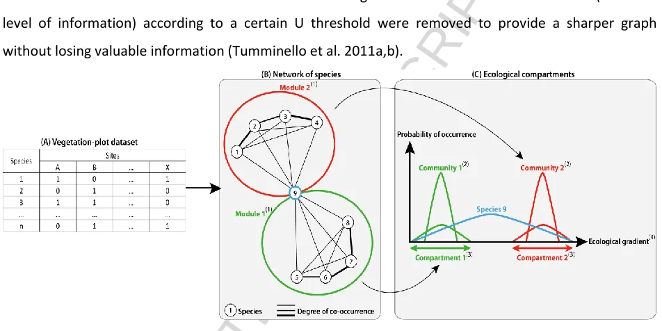
The co-occurrences between pairs of species were derived from the vegetation-plot dataset. They were then translated into a graph where the nodes represent each species and the thickness of edges represents the degree of co-occurrence between pairs of species (

Figure 2). We used the U index (Bruelheide 2000) as a statistical measure of co-occurrence (edge weight) instead of the exact co-occurrence within the dataset. Edges with a low level of co-occurrence (i.e. a low level of information) according to a certain U threshold were removed to provide a sharper graph without losing valuable information (Tumminello et al. 2011a,b).

Figure 2: Construction of a network of species from vegetation-plot data and ecological interpretation: (A) vegetation-plot dataset consists of sites/species tables with presence/absence data; (B) an index of co-occurrence between pairs of species (U) is computed from the table and allows a network to be constructed: the nodes represent each species and the edge thicknesses the index U; (C) here the structure of the network is assumed to be caused by ecological requirements of species: each cluster of nodes (representing species with similar ecological requirements), called module (1), is a representation of plant communities (2) based on their ecological affinities. These communities can then be associated with specific ecological compartments (3) along ecological gradients (4).

Co-occurrence of pairs of species within a particular plot is assumed to be caused mainly by the same or similar ecological requirements (

Figure 2 (C); i.e. habitat filtering, Lortie et al. 2004) with no detection of biotic interactions between species (biotic filtering). In this way using graph theory enables identification of groups of species based on ecological affinities.

real-ACCEPTED MANUSCRIPT

6

world communities rather than species from other modules because they share similar ecological requirements.

A second level of analysis of a graph structure is to analyse in more detail the role of each node (species) according to their pattern of intra- and inter-module connections (Guimerà and Amaral 2005). They define a within module degree (z) which measures how well-connected is a vertex to other vertices inside the module and a participation coefficient (C) which measures how well-distributed the edges of a vertex are among other modules. A species with both high z and low C - called ‘provincial hubs’ - is believed to be a good indicator of module habitats conditions (i.e. called here ecological compartment) because it shares ecological requirements with many other species of the same module. We expected these species to be widely distributed among plant communities inside this particular ecological compartment, whereas species with low z and C – called ‘peripheral hubs’– have stronger ecological requirements and are very likely to occur in more specialized plant communities in more constrained ecological sub-compartments. This ratio z/C is particularly interesting when studying species strategies (ubiquist/endemic/indicator) and will help us choose the most ‘provincial’ species to represent best the ecological behaviour of each module.

III.2.Ecological gradients

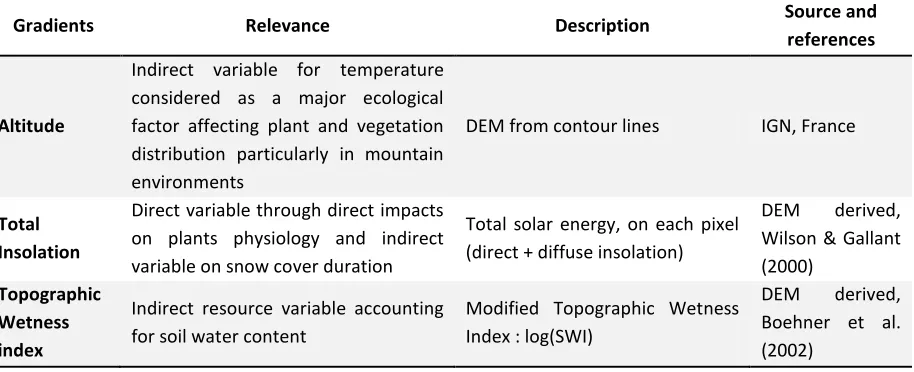
A small set of continuous ecological variables (Table 1) was recognized to affect spatial distribution of grasslands alpine species at the mapping scale used (25 m grid resolution on 5,000 Km² of study area). Plot size (4-50 m²) is smaller than variable resolution (25*25 m) but we assumed here the spatial homogeneity of species assemblages at the pixel level. Therefore, species-environment relationships and variability were well-captured at this resolution.

Table 1: Ecological gradients used to characterize species-environment relationships for the species distribution models (SDMs). All variables have a 25m resolution (grid, raster)

Gradients Relevance Description Source and

references

Altitude

Indirect variable for temperature considered as a major ecological factor affecting plant and vegetation distribution particularly in mountain environments

DEM from contour lines IGN, France

Total Insolation

Direct variable through direct impacts on plants physiology and indirect variable on snow cover duration

Total solar energy, on each pixel (direct + diffuse insolation)

DEM derived, Wilson & Gallant (2000)

Topographic Wetness index

Indirect resource variable accounting for soil water content

Modified Topographic Wetness Index : log(SWI)

ACCEPTED MANUSCRIPT

7

Degree of

convexity

Indirect variable affecting snow cover duration, local temperature and wind conditions

Topographic analysis : radius of 50m for micro-topography, radius of 500m for main relief features

DEM derived, Weiss (2001)

Spatial dependence

Climatic gradient across study area

(NW/SE gradient) log(latitude/longitude)

Derived from localisation

III.3.Modelling platform

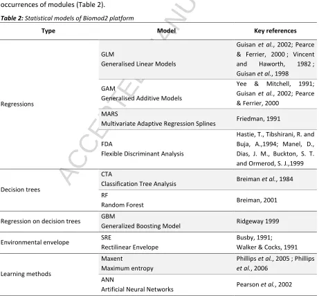
We used a multi-modelling platform, Biomod2 (see Thuiller et al. 2009; Thuiller et al, 2013), which allowed the use of 10 statistical models to calibrate the relationship between explanatory variables and occurrences of modules (Table 2).

Table 2: Statistical models of Biomod2 platform

Type Model Key references

Regressions

GLM

Generalised Linear Models

Guisan et al., 2002; Pearce & Ferrier, 2000 ; Vincent and Haworth, 1982 ; Guisan et al., 1998

GAM

Generalised Additive Models

Yee & Mitchell, 1991; Guisan et al., 2002; Pearce & Ferrier, 2000

MARS

Multivariate Adaptive Regression Splines Friedman, 1991

FDA

Flexible Discriminant Analysis

Hastie, T., Tibshirani, R. and Buja, A.,1994; Manel, D., Dias, J. M., Buckton, S. T. and Ormerod, S. J.,1999

Decision trees

CTA

Classification Tree Analysis Breiman et al., 1984 RF

Random Forest Breiman, 2001

Regression on decision trees GBM

Generalized Boosting Model Ridgeway 1999

Environmental envelope SRE

Rectilinear Envelope

Busby, 1991;

Walker & Cocks, 1991

Learning methods

Maxent

Maximum entropy

Phillips et al., 2005 ; Phillips et al., 2006

ANN

ACCEPTED MANUSCRIPT

8

The resulting models were compared based on their relative performance in fitting the observed data (Elith et al. 2006). A first statistical assessment was performed using ROC sensitivity analysis, which was calculated for each model on 1,000 repetitions using 75 per cent of the sampled data. Statistical assessment was also supported with expert assessments conducted on the final distribution maps. Both outcomes were combined to produce the best distribution models that were used at the end for mapping ecological compartments.

IV.

Results

IV.1.Species network

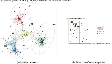
Figure 3 shows the resulting network derived from vegetation-plot data after application of the co-occurrence index (U) threshold and filtering on siliceous alpine grasslands species. The U index value –

empirically set to 15 – results from a trade-off between (i) an excessive amount of low-level information (i.e. low U, poorly-connected species) but high number of species and (ii) high-level information (i.e. high U, highly-connected species) but low number of species. Modules 1 and 3 are very sharp owing to species with very low participation coefficient on average. Modules 2, 4 and 5 are fairly sharp with relatively higher participation coefficients. Module 6 is significantly connected to its neighbours through

‘connector-hub’ species and, therefore, was not modelled. For each module, species showing the best C/z profile (low C and high z) were selected as indicator species.

ACCEPTED MANUSCRIPT

9

parameter space helps characterize each species and module role in the network; central species are chosen within the upper left square of provincial hubs (I). Following and simplifying Guimerà and Amaral (2005) other principal roles of nodes are peripheral nodes (II), connector hubs (III i.e. module 6) and non-hub connector (IV).

Species inside a module are linked with each other by their ecological affinities (common niche) and not by botanical characteristics, supporting the use of ecological datasets to predict vegetation potential distribution.

IV.2.Modules, ecological compartments and indicator species

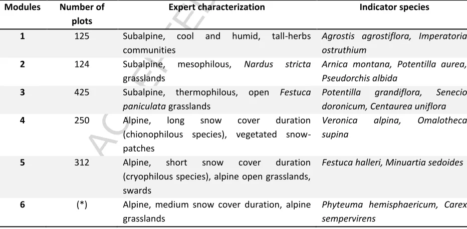
Based on a modularity analysis and on an expert examination of the resulting species’ network, 5 assemblages (M1, M2, M3, M4, M5) were selected (Table 3) for their wide representation in the field, their botanical consistency and their ecological dissimilarities. The modules are exclusive and therefore, in the modelling process, the presence points of a specified module were considered as absence points for all other modules.

Table 3: Expert characterization of modules yielded by the infomap modularity analysis and indicator species. (*) Module 6 was not modelled, providing its transitional positioning (high C value of species); the resulting ecological compartment strongly overlaps with the ones of other modules.

Modules Number of

plots

Expert characterization Indicator species

1 125 Subalpine, cool and humid, tall-herbs communities

Agrostis agrostiflora, Imperatoria ostruthium

2 124 Subalpine, mesophilous, Nardus stricta grasslands

Arnica montana, Potentilla aurea, Pseudorchis albida

3 425 Subalpine, thermophilous, open Festuca paniculata grasslands

Potentilla grandiflora, Senecio doronicum, Centaurea uniflora 4 250 Alpine, long snow cover duration

(chionophilous species), vegetated snow-patches

Veronica alpina, Omalotheca supina

5 312 Alpine, short snow cover duration (cryophilous species), alpine open grasslands, swards

Festuca halleri, Minuartia sedoides

6 (*) Alpine, medium snow cover duration, alpine grasslands

Phyteuma hemisphaericum, Carex sempervirens

IV.3.Modelling results

ACCEPTED MANUSCRIPT

10

Four types of models showed ROC cut-off values above 0.85 – the threshold above which a model is considered here to have a good sensitivity or sufficient statistical relevance. The models that performed best were a GLM and a GAM, an RF, a GBM and a MaxEnt (see Table 2). The GLM successfully handled the expert assessment stage because it provided maps with both consistent probability levels and spatial extent closest to reality. MaxEnt also showed good spatial extent but low-probability levels whereas other types of models showed a trend to either over-estimate or limit spatial extent. For all models, around 80 per cent of presence data were properly predicted on average (sensitivity relevant) with relatively weak differences among modules. The same percentage and pattern were properly predicted for absences data. The importance of variables was in agreement with expert knowledge and underlined altitude as the key ecological factor influencing species-environment relationships. Close examination of the importance of variables is, nevertheless, beyond the scope of this proceedings paper. It is worth noticing that the degree of convexity at small scale (radius of 50m) did not show any statistical significance.

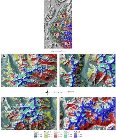
IV.4.Resulting map

At the end, all best-performing models (only GLMs) were mapped together (Figure 4). Each grid-cell was

assigned to the model with the highest probability only if the differences with all other modules’

probabilities were higher than 0.2. Otherwise, if the difference with another module was lower than 0.2 it was labelled as an overlap grid-cell (not shown here). Thus, the map represents the cores of the ecological compartments. Probabilities lower than 0.5, indicating a weak probability of occurrence; have clearer colours on the map in order to identify the zones of modelling uncertainty.

ACCEPTED MANUSCRIPT

11

ACCEPTED MANUSCRIPT

12

V.

Discussion

Application of graph theory to vegetation-plot data combined with species distribution models has revealed ecologically-coherent species’ assemblages and consistent ecological compartments’

distribution. Compared to classical ecological clustering using environmental data, this modelling

method yields ecological compartments that take into account vegetation’s ecological requirements. This approach was successful to reveal gradual changes in environmental conditions: probabilities gently follow the topographic gradients, which are typically marked in the mountain environment. The transitional zones (i.e. the overlaps between ecological compartments) which represent 22.5 % of the area were in most cases ecologically relevant. The most frequently found were the transition between nival and cryophilous conditions (between modules 4 and 5: alpine belt) and the transition between mesophilous and thermophilic conditions (modules 2 and 3: subalpine belt).

Applying SDM at the landscape scale using explanatory variables derived from Digital Elevation Model (DEM) with a resolution of 25 m is quite rare in the literature. However, these variables, chosen to be

close to plants’ direct resources (e.g. total insolation for solar energy or topographic wetness index for

soil water content) and generics for plants’ pattern delineation in mountains’ environments, are relevant

to predict ecological compartments. Besides, it makes it useful to vegetation scientists because at this scale predictive maps are close to their on-ground perception.

Significant explanatory variables of species’ assemblages’ distributions are in accordance with our

models. Altitude and total solar radiation were the most important variables, followed by the large-scale topographic position (convexity with radius of 500m). The spatial dependence variable played also a significant role, especially in the delineation of thermophilic subalpine ecological compartment (module 3) as it occurs much more in the southern part of the area. The small-scale topographic position (convexity with radius of 50m) seemed not to account for micro-topographic patterns due in part to the mismatch of resolution with the DEM used (25 m). Thus, a high resolution DEM will be very helpful in the near future to improve fine-scale distribution patterns. Another improvement would be the use of a time

series’ analysis of NDVI (Normalized Difference Vegetation Index) images that would allow a better

evaluation of the snow cover and the different phenologies of vegetation.

The approach here allows optimizing time and field efforts to map vegetation in complex mountain areas. In particular, it will serve as key input within the framework of CarHab project, by providing

ACCEPTED MANUSCRIPT

13

In all, graph theory has proven to be suitable to analyse vegetation-plot data under a community-based approach and to propose species assemblages as objects to be modelled across complex landscapes. When vegetation data are available, using SDM with well-defined indicator species in addition to simple and generic explanatory variables allows the production of relevant ecological compartments in

conformity with fields’ expert knowledge.

VI.

Acknowledgments

This work was partly funded by the French Ministry of Ecology, Sustainable Development and Energy in support of the development of the CARHab project (2011-2015) on mapping the terrestrial habitats of France. In addition, this work benefited from a synergy with the Divgrass project (Plant Functional Diversity of Permanent Grasslands) (CESAB/FRB funded, France) and exchanges with Dr. Philippe Choler (Divgrass PI).

VII.

References

1. Boehner, J., Koethe, R., Conrad, O., Gross, J., Ringeler, & A., Selige, T. (2002). Soil Regionalisation by Means of Terrain Analysis and Process Parameterisation. In: Micheli, E., Nachtergaele, F., Montanarella, L. [Ed.]: Soil Classification 2002. European Soil Bureau, Research Report No. 7, EUR 20398 EN, Luxembourg, 213-222.

2. Breiman, L., Friedman, J., Stone, Ch. J, & Olshen, R.A. (1984). Classification and regression trees. Chapman and Hall.

3. Breiman, L. (2001). Random forests. Mach. Learn. 45, 5-32.

4. Brown, J. H., & Lomolino, M. V. (1998). Biogeography (2nd ed). Sunderland MA, Sinauer Associates. 5. Bruelheide, H. (2000). A new measure of fidelity and its application to defining species groups.

Journal of Vegetation Science, 11(2), 167-178.

6. Busby, J.R. (1991). BIOCLIM: A bioclimate analysis and prediction system. In: Margules, C.R. (Ed.), Nature Conservation: Cost Effective Biological Surveys and Data Analysis. CSIRO, Australia, 64–68. 7. Dale, M. (1977a). Graph theoretical analysis of the phytosociological structure of plant communities

– the theoretical basis. Vegetatio 34 (3), 137-154.

8. Dale, M. (1977b). Graph theoretical analysis of the phytosociological structure of plant communities

– an application to mixed forest. Vegetatio 35 (1), 35-46.

9. EEA (European Environmental Agency) (2014). Technical Report Habitat and vegetation mapping in Europe - an overview. MNHN-EEA report N1/2014, 163 Pages.

http://spn.mnhn.fr/spn_rapports/archivage_rapports/2014/SPN%202014%20-%2010%20-%20Terrestrial_habitat_mapping_in_Europe_-_an_overview.pdf

10. Elith, J., Guisan, A., Hijmans, R. J, Huettmann, F., Leathwick, J. R, Lehmann, A., Li, J., Lohmann, L. G, Anderson, R. P, & Dudík, M. (2006). Novel Methods Improve Prediction of Species’ Distributions

from Occurrence Data. Ecography, 29(2), 129-151.

11. Ferrier, S., Drielsma, M., Manion, G., & Watson, G. (2002). Extended statistical approaches to modelling spatial pattern in biodiversity in northeast New South Wales. II. Community-level modelling. Biodiversity and Conservation, 11(12), 2309-2338.

12. Friedman, J. (1991). Multivariate adaptive regression splines. Ann. Stat. 19, 1-141.

13. Funk, V. A., & Richardson, K. S. (2002). Systematic data in biodiversity studies: use it or lose it.

ACCEPTED MANUSCRIPT

14

14. Graham, C. H., & Hijmans, R. J. (2006). A comparison of methods for mapping species ranges and species richness. Global Ecology and Biogeography, 15(6), 578-587.

15. Guimera, R., & Amaral, L. (2005). Functional cartography of complex metabolic networks. Nature, 433(7028), 895-900.

16. Guisan, A., Theurillat, J. P. & Kienast, F. (1998). Predicting the potential distribution of plant species in an alpine environment. J. Veg. Sci., 9, 65-74.

17. Guisan, A., Edwards, T.C., & Hastie, T. (2002). Generalized linear and generalized additive models in studies of species distributions: setting the scene. Ecological Modelling, 157, 89–100.

18. Hastie, T., Tibshirani, R. & Buja, A. (1994). Flexible discriminant analysis by optimal scoring. J. Am. Stat. Assoc., 89, 1255-1270.

19. Lortie, C. J., Brooker, R. W., Choler, P., Kikvidze, Z., Michalet, R., Pugnaire, F. I., & Callaway, R. M. (2004). Rethinking plant community theory. Oikos, 107(2), 433-438.

20. Manel, D., Dias, J. M., Buckton, S. T. & Ormerod, S. J. (1999). Alternative methods for predicting species distribution: an illustration with Himalayan river birds. Journal of Applied Ecology, 36, 734-747.

21. Pearce, J., & Ferrier, S. (2000). Evaluating the predictive performance of habitat models developed using logistic regression. Ecological Modelling, 133, 225–245.

22. Pearson, R.G., Dawson, T., Berry, P., & Harrison, P. (2002). SPECIES: a spatial evaluation of climate impact on the envelope of species. Ecological Modelling, 154, 289–300.

23. Peterson, A.T. (2007). Uses and requirements of ecological niche models and related distributional models. Biodiversity Informatics, 3, 59–72.

24. Phillips, S.J., Anderson, R.P., & Schapired, R.E. (2005). Maxent software for species distribution modeling. AT&T Labs-Research, Princeton University, Center for Biodiversity and Conservation, American Museum of Natural History.

25. Phillips, S.J., Anderson, R.P., & Schapire, R.E. (2006). Maximum entropy modeling of species geographic distributions. Ecological Modelling, 190, 231–259.

26. Proulx, S. R., Promislow, D. E., & Phillips, P. C. (2005). Network thinking in ecology and evolution.

Trends in Ecology & Evolution, 20(6), 345-353.

27. Ricklefs, R. E. (2004). A comprehensive framework for global patterns in biodiversity. Ecology Letters, 7(1), 1-15.

28. Ridgeway, G. (1999). The state of boosting. Comput. Sci. Stat., 31, 172-181.

29. Rosenzweig, M. L. (1995). Species diversity in space and time. Cambridge University Press.

30. Rosvall, M., & Bergstrom, C. T. (2008). Maps of random walks on complex networks reveal community structure. Proceedings of the National Academy of Sciences, 105(4), 1118-1123.

31. Rushton, S. P., Ormerod, S. J., & Kerby, G. (2004). New paradigms for modelling species distributions?. Journal of Applied Ecology, 41(2), 193-200.

32. Thuiller, W., B. Lafourcade, R. Engler, & M. B. Araújo (2009). BIOMOD–a Platform for Ensemble Forecasting of Species Distributions. Ecography, 32(3), 369–73.

33. Thuiller, W., Georges, D., & Engler, R. (2013). biomod2: Ensemble platform for species distribution modeling. R package version, 2(7), r560.

34. Tumminello, M., Miccichè, S., Lillo, F., Piilo, J., & Mantegna, R. N. (2011a). Statistically validated networks in bipartite complex systems. PloS one, 6(3), e17994.

35. Tumminello, M., Miccichè, S., Lillo, F., Varho, J., Piilo, J., & Mantegna, R. N. (2011b). Community characterization of heterogeneous complex systems. Journal of Statistical Mechanics: Theory and Experiment, 2011(01), P01019.

ACCEPTED MANUSCRIPT

15

37. Walker, P. A., & Cocks, K. D. (1991). HABITAT - a Procedure for Modeling a Disjoint Environmental Envelope for a Plant or Animal Species. Global Ecology and Biogeography Letters, 1, 108-118.

38. Weiss, A. D. (2001). Topographic Position Index and Landforms Classification. Poster Presentation, ESRI Users Conference, San Diego, CA

39. Wilson, J. P., & Gallant, J. C. (Eds.). (2000). Terrain analysis: principles and applications. John Wiley & Sons.

40. Yarrangton, G. A. (1973). A Graph theoretical test of phytosociological homogeneity. Vegetatio, 28(5-6), 283-298.

ACCEPTED MANUSCRIPT

16

ACCEPTED MANUSCRIPT

17

Highlights (max 85 characters per bullet point, including spaces)

 species’ geographic distributions supports conservation planning and forecasting

 mapping natural and semi-natural habitats of complex mountain vegetation mosaics

 Spatial approach provides different alternatives for policy makers to help conservation targets

 we propose species assemblages as objects to be modelled across complex landscapes