Portfolio Mathematics with General Linear and Quadratic Constraints

(1)

https://www.scirp.org/journal/jmf ISSN Online: 2162-2442 ISSN Print: 2162-2434

DOI: 10.4236/jmf.2019.94034 Oct. 30, 2019 675 Journal of Mathematical Finance

Portfolio Mathematics with General

Linear and Quadratic Constraints

David L. Stowe

Department of Finance, Ohio University, Athens, Ohio, USA

Abstract

This paper explores the mathematics behind optimal portfolio construction when relative utility and risk are considered together in a general sense. I de-rive the portfolio optimization problems when subject to both a general liner constraint and a constraint to tracking error (a quadratic constraint), the most pervasive constraint placed on delegated portfolio managers. This un-ifies three very influential papers from the evolution of optimal portfolio theory. In addition, I also analyze the general linear constraint when applied to Sharpe Ratio maximization. When applied together, these formulations can allow principals and agents to better analyze alternatives and negotiate contracting in order to ensure that the constraints generate proper utility maximization.

Keywords

Portfolio Mathematics, Optimization, Delegated Portfolio Management, Tracking Error, Utility Maximization

1. Introduction

The purpose of this essay is to generalize the Markowitz portfolio choice prob-lem and derive solutions to the variance minimization and utility maximization problems considering both general linear constraints and a single quadratic con-straint. The Markowitz portfolio choice problem (introduced in [1]) has been studied from many different perspectives. The problem is essential to minimize the variance of a linearly combined set of correlated random variables (returns), conditioned on the mean of these variables, with a constraint on the scalers or weights. The set of all such points is called the efficient frontier, i.e. the mini-mum variance envelope. The modern expression of the optimization problem outlined by Markowitz is due to Merton [2] who derives the solutions analyti-How to cite this paper: Stowe, D.L. (2019)

Portfolio Mathematics with General Linear and Quadratic Constraints. Journal of Ma-thematical Finance, 9, 675-690.

https://doi.org/10.4236/jmf.2019.94034

Received: July 12, 2019 Accepted: October 27, 2019 Published: October 30, 2019 Copyright © 2019 by author(s) and Scientific Research Publishing Inc. This work is licensed under the Creative Commons Attribution International License (CC BY 4.0).

(2)

DOI: 10.4236/jmf.2019.94034 676 Journal of Mathematical Finance

cally using linear algebra. His solution considers the problem as a quadratic programming problem with two predefined linear constraints, the weight con-straint (scalar concon-straint) and the expected return concon-straint (the mean). The statement of the problem is as follows. Matrices and vectors are in boldface.

w - n × 1 weight vector of the portfolio.

Ω - n × n covariance matrix (symmetric and positive definite). r - n × 1 vector of expected returns.

1 - n × 1 vector of 1’s.

min ′ s.t. ′ =1 and ′ =r.

w wΩw w1 w r (1.1) However, the problem can also be solved with a general linear constraint as demonstrated by Best and Grauer [3]. The general linear constraint opens up possibilities to make considerations for and constraints on portfolio beta, sector or industry weights, multi-stage optimization, etc. I derive the solution to the general linear constraint problem in part 2 of this essay to familiarize the reader with my notation and so I can use it in my derivation of the maximum Sharpe Ratio problem.

However, since the original introduction of the model, modern thinking on portfolio construction (and financial theory in general) has evolved to consider the differences in incentives between the individual making the portfolio choices, the agent, and the individual hiring the delegated manager, the principal. This spawned a theory of active portfolio management, or delegated portfolio man-agement, which centers on a time series of excess returns, essentially the returns of a security or portfolio in excess of a benchmark. This is a space transforma-tion that causes agents to optimize in excess return space rather than raw return space (or even another excess return space with a different benchmark). Princip-als are then potentially motivated to constrain agent behavior in this space by putting limits on the variance of the delegated manager’s excess return, i.e. their tracking error variance.

There are many modern examples of papers analyzing delegated or relative problems. Bisburgen, Brandt, and Koijen [4] revisit the problem of multiple ex-ternal agents relaxing the assumption about the certainty of the agents’ risk ap-petites and conclude that serious inefficiency exists without this assumption. Blake et al. [5] use the BBK framework and apply it to the delegated relation-ships in the pension industry and, among many other things, show that the de-legated incentive is pervasive in professional investment management. Cuoco and Kaniel [6] analyze the linkage between compensation contracts and excess performance in delegated portfolio management. However, the delegated con-tracting problem can probably best be summed up by analyzing the tracking er-ror constraint.

(3)

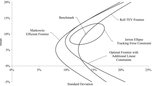
applies a tracking error constraint to a mean/variance optimization problem, thus introducing a quadratic constraint into the problem. Whereas the Marko-witz problem, under linear constraints, forms a minimum variance set shaped like a parabola in mean and variance, the tracking error constraint causes the ef-ficient set to be shaped like an ellipse, with the feasible portfolios inside. See Figure 1 for a visual example of these curves.

The closest application of a utility problem directly to Roll’s TEV frontier by Bertrand [9]. In this paper, he considers the problem of a fixed risk aversion constraint in mean/variance and its ability to generate preferred portfolios.

The variance minimization problem is one approach to analyzing portfolio choice. However, it is also reasonable to consider the problem of maximizing utility. The popular utility function considered in this problem is a “quadrat-ic-style” utility where the investor’s utility increases in the expected return, w r′ ,

and decreases in the expected risk or variance, w′Ωw. And, the parameter, a,

measures the sensitivity or the tradeoff: the level of risk aversion. The relation-ship is expressed as follows:

max ′ −a ′ w

w r wΩw (1.2)

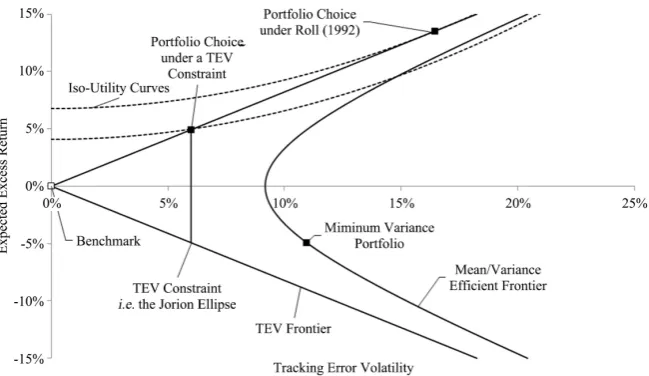
Figure 2 shows a few of the curves depicted in Figure 1 with iso-utility curves corresponding to the same level of risk aversion, a.

Modern extensions of the Markowitz portfolio choice problem tend to focus more on altering something fundamental about the model or analyzing a specific constraint. For example, Chen et al. [10] optimize over semivariance but the model is adjusted to account for uncertainty in variable estimation based on historical data. Or authors may use modern techniques to analyze traditional problems like Kar et al. [11] that optimizes over the Sharpe Ratio and the Value at Risk simultaneously. These papers are very interesting and practical consider-ations for real world applicconsider-ations of this theory.

(4)

[image:4.595.137.462.71.256.2]

DOI: 10.4236/jmf.2019.94034 678 Journal of Mathematical Finance Figure 1. Optimal sets in mean/standard deviation space given differing constraints. This figure

depicts mean/standard deviation space. The three curves open to the right are hyperbolas. They are solutions to quadratic programming problems with linear constraints. Notably, if the hori-zontal axis were in variance, these would be parabolas, and the circular shape would be an el-lipse. The furthest curve to the left is the minimum variance envelope derived my Markowitz [1]. The next curve is a Markowitz minimization problem with additional linear constraints (a beta constraint in this case). The point labeled Benchmark is a portfolio that an arbitrary dele-gated investment manager would be given. The curve passing through the benchmark is the minimum tracking error curve, the TEV Frontier, derived by Roll [7]. The ellipse is the optimi-zation of the Markowitz problem subject to tracking error constraint (a quadratic constraint) as proposed in Jorion [8].

[image:4.595.136.463.413.593.2]

(5)

2. Mean/Variance Optimization with a General Linear

Constraint

The general linear constraint problem analyzed in Best and Grauer [3] comes in two forms, variance minimization given linear constraints and utility maximiza-tion given linear constraints. Although these problems are already solved, I re-peat this calculation to familiarize the reader with my notation and so I can refer to my solutions throughout the paper. Additionally, I leave the expressions in the purest form possible, without making extraneous substitution. As before, the notation used throughout this paper is as follows:

w - n × 1 weight vector of the portfolio.

Ω - n × n covariance matrix (symmetric and positive definite). E - n × k matrix of constraint conditions.

c - 1 × k vector of constraint constants.

2.1. Minimize Variance with a General Linear Constraint

The variance function with a weight vector and a covariance matrix is w′Ωw.

We want to minimize this function given a general linear constraint on the weights as follows:

min ′ s.t. ′ = . w wΩw w E c

We introduce a new vector, Λ_{, to use as Lagrange multipliers:} Λ - k × 1 vector of Lagrange multipliers.

The Lagrangian is:

(

)

.

L=w′Ωw− w E′ −c Λ

We differentiate the Lagrangian and set it equal to zero to find the critical values:

2Ωw−EΛ=0.

Solving for the weight vector yields: 1

1

. 2

−

=

w Ω EΛ

Next, we plug this weight vector into the condition to solve for the Lagrange multipliers:

1

. 2

−

′ = ′ ′ =

w E Λ ΩE E c

(

)

1

2 ′ − − ′.

= E E c

Λ Ω

Plugging this value into the expression for the weight vector above reveals the optimal weight vector given the general linear constraint:

(

)

1

1 1

.

−

− _′ − _′

=

w Ω E EΩ E c (2.1.1)

(6)

(

₁

)

1

.

− −

′ = ′ ′

wΩw c EΩ E c

This is an equally beautiful expression. To solve this with the Markowitz con-straints from Equation (1.1), we would make:

[

]

,

=

E 1 r

and

1 .

r   =    

c

E is essentially an augmented matrix with a column of 1s and a column of ex-pected returns for each security. c is a 2 × 1 matrix where the constraint on the top represents the sum of all the weights equaling 1 and the bottom r representing the sum of all the weights times the expected returns equaling a target weight, the weighted average expected return. The expression of the Mar-kowitz minimum variance envelope with these constraints is:

[

]

1

[

]

1

1 1

.

r r

− −

′

  _ _′ _  

′ _{=  } _ _ _{ }

 

   

wΩw 1 r Ω 1 r

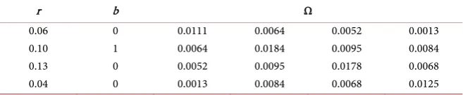
And, we can vary the constraint, r, to trace out the entire frontier as depicted in Figure 1. Table 1 includes the parameters used to make the calculations in the figures.

2.2. Maximize Utility with a General Linear Constraint

The utility function in Equation (1.2) can also be computed with a general linear constraint. This form of utility is particularly convenient because it is expressed as a quadratic programming problem. We introduce a new constant into this utility, the risk aversion level, which is essentially the slope of the utility function (in variance) and reintroduce the return vector:

a - level of risk aversion.

r - n × 1 vector of expected returns. The problem is as follows:

max ′ −a ′ s.t. ′ = . w w r wΩw w E c We set up the Lagrangian:

(

)

.

[image:6.595.210.539.623.691.2]

L=w r′ −aw′Ωw− w E′ −c Λ

Table 1.Numerical values used to build the figures.

r b Ω

0.06 0.10 0.13 0.04

0 1 0 0

0.0111 0.0064 0.0052 0.0013

0.0064 0.0184 0.0095 0.0084

0.0052 0.0095 0.0178 0.0068

(7)

Differentiate the function and set the conditions to zero:

2a .

− − =

r Ωw EΛ 0

Solve for the weight vector:

(

)

1

. 2a

−

= −

w Ω r EΛ

Reapply the constraint condition to calculate Λ:

(

)

1

. 2a

−

′

′ = − =

w E r EΛ Ω E c

(

) (

1

)

1 1

2a .

−

− −

′ ′ ′

= E E E r− c

Λ Ω Ω

And lastly, plug Λ into the weight vector, do some rearranging, and this yields the optimal weights:

(

)

1

(

)

1

)

1 1 1 1 1 1

. 2a

− −

− _′ − _′ − _′ − _′ −

= + −

w Ω E EΩ E c Ω r E EΩ E EΩ r (2.2.1)

This expression is messier than above but after the rearranging, one can see that the final solution in Equation (2.2.1) is simply the minimum variance solu-tion from Equasolu-tion (2.1.1) shifted by an addisolu-tional term.

2.3. Optimize in Excess Return/Tracking Error

The problem proposed by Roll [7] suggests that delegated managers optimize in excess return/tracking error volatility (TEV) rather than mean/variance. The solutions to these problems are identical to the solutions derived in sections 2.1 and 2.2 albeit with a different weight vector and different constraints. We need to introduce another weight vector into the process:

b - n × 1 constant vector of weights (for a benchmark).

Tracking error variance and excess return are then defined as follows:

(

_w₋_b

) (

′_Ω _w₋_b

)

_{- Tracking error variance (TEV).}

(

_w₋_{b r}

)

′ _{- Excess return.}

Since b is a constant vector, we could substitute it into any of the expressions in 2.1 and 2.2 and still have a valid derivation. Thus, similar to Equation (2.1.1), the weight vector that solves the TEV minimization problem:

(

) (

)

(

)

min − ′ − s.t. − ′ = .

w w b Ω w b w b E c

is:

(

)

₁

(

₁

)

1

.

−

− _′ − _′

− =

w b Ω E EΩ E c (2.3.1)

And, the weight vector that solves a utility maximization problem:

(

)

(

) (

)

(

)

max − ′ −a − ′ − s.t. − ′ = .

w w b r w b Ω w b w b E c

is:

(

)

₁

(

₁

)

1 1 ₁

(

₁

)

1 ₁

)

. 2a

− −

− _′ − _′ − _′ − _′ −

− = + −

w b Ω E EΩ E c Ω r E EΩ E EΩ r (2.3.2)

(8)

change slightly. To replicate the solutions in Roll (1992), the constraint vector needs to be set as follows:

0 .

w b

r r

 

=  ₋ 

 

c

Taken the two vectors, w and b, which should each normalize to 1, their dif-ference is 0. Also the second constraint is now the excess return constraint,

w b

r −r , in order to draw the curves appropriately. See Figure 3 for a representa-tion of these curves drawn in tracking error space.

[image:8.595.212.537.418.606.2]

3. Optimize with an Additional Tracking Error Constraint

The variance optimization problem given a tracking error constraint was origi-nally solved in the context of portfolio choice in Jorion [8]. In this framework, he used the standard Markowitz constraints, the length of the weight vector and the weighted average expected return, to derive an ellipse in mean/variance space inside of which contains all portfolios with tracking error less than the constraint. In this section, which is the primary contribution of this essay, I de-rive “Jorion’s ellipse” with the general linear constraint of Best and Grauer [3]. This contribution unifies the analysis of linear constraints on the portfolio opti-mization model and the significance of relative portfolio optiopti-mization to modern delegated contracting. The closed-form nature of these solutions gives analysts a conceptual, theoretical framework to perform comparative analysis without having to rely on numerical simulation.

(9)

3.1. Optimize Var with General Linear and Tracking Error Constraints

As with before, we will need a couple new variable definitions: 2

T - Tracking error variance constraint.

λ_{- Lagrange multiplier for the tracking error constraint.} We, once again, begin by stating the problem:

(

) (

)

2

min ′ s.t. ′ = , − ′ − =T .

w wΩw w E c w b Ω w b The Lagrangian then follows:

(

)

(

) (

)

2

)

.

L=w′Ωw− w E′ −c Λ−λ w−b ′Ω w− −b T

Next we differentiate by w as set the resulting equations equal to zero:

(

)

2Ωw−EΛ−λ 2Ωw−2Ωb =0.

Solving for w yields the following vector:

(

1

)

1

(

2

)

.

2 1 λ λ

−

= −

−

w Ω EΛ Ωb

Applying the first constraint allows us to calculate one of the Lagrangian terms, Λ_:

(

1

) (

2

)

1 .

2 1 λ λ

−

′ = ′ ′− ′ =

−

w E ΛE bΩ Ω E c

(

)

1

(

)

1

2 1 λ 2λ .

− −

′ ′ ′

= E E − c + E b

Λ Ω

Substituting Λ_{back into the vector for w yields:}

(

)

1

(

)

1

)

1 1 1 1

. 1 λ λ − − − _′ − _′ − _′ − _′ = + − −

w Ω E EΩ E c Ω E EΩ E E b b

Because the second condition is easier to calculate if we consider the vector (w – b), we can subtract b from the vector above:

(

)

(

₁

(

₁

)

1

)

(

₁

(

₁

)

1

)

. 1 λ λ − − − _′ − _′ − _′ − _′ − = − + − −

w b Ω E EΩ E c b Ω E EΩ E E b b

Applying the condition yields the following equation, after some minor sim-plification:

(

) (

)

(

)

(

)

(

)

(

)

(

)

(

)

2 1 2 1 1 2 1 1 1

1 1 2

2 1 2 1 2 . b b b T λ _σ λ λ _σ λ σ − − − − − − − − ′ − −   _′ _′ _′ =_ _ − −     _′ _′ _′ + _ _ − −   ′ ′ ′ ′ ′ + − + =

w b w b

b E E E E b

c E E c b E E E c

Ω

Ω Ω

where 2 b

(10)

Lastly, after some profuse and tedious elementary algebra, and an application of the quadratic equation, the constant can be solved for:

(

)

(

)

(

)

1 2 1

1 2 2

1

2 1

2

1 1 .

1 b b T σ λ λ _σ − − − −  ₊ _′ _′ _′₋ ₊   _{= − ± −}_ _  ₋  _ _   _ − ′ ′ ′ _

c b E E E c

b E E E E b

Ω Ω

And the optimal solution for w is obtained by plugging in the constant:

(

)

(

)

(

)

(

)

(

)

(

)

1 1 1 1 2 1

1 2 2

1 2 1 1 1 1 2 1 1 . b b T σ σ − − − − − − − − − − ′ ′ =  _ _′ _′ _′ _  + − +  _ _  − ± −_ _ _ _  − ′ ′ ′   _ _    ′ ′ ⋅ −

w E E E c

c b E E E c

b E E E E b

E E E E b b

Ω Ω

Ω Ω Ω Ω

(3.1.1)

This weight vector is the solution to the problem of optimizing variance given a general linear and a tracking error constraint. Additionally, as before, this vec-tor is a transformation of the general minimum variance solution shifted by a term in two directions. The ± draws out half of the curve in one direction and the other half in the other direction. The linear constraints in combination with the tracking error constraint can cause there to be an infinite number, two, one or no real solutions to the problem. It is certainly notable that the two con-straints can work in conflict and generate imaginary vectors. Essentially, if the linear constraints generate a curve that doesn’t pass through the tracking error constrained ellipse, then there will be no real solutions to this problem.

3.2. Optimize Utility Given General Linear & Tracking Error Constraints

The utility optimization problem can also be important to principals. Knowing the best possible outcome given a tracking error constraint could be a useful metric when deciding how strict to make this constraint. No new variables are needed. The statement of the problem is as follows:

(

) (

)

2

max ′ −a ′ s.t. ′ = , − ′ − =T .

w w r wΩw w E c w b Ω w b The Lagrangian is then set up:

(

)

(

) (

)

2

)

.

L=w r′ −aw′Ωw− w E′ −c Λ−λ w−b′Ω w− −b T

Then it is differentiated and set to zero:

(

)

2a 2λ .

− − − − =

r Ωw EΛ Ωw Ωb 0

Before moving to the next step, it is convenient to add 2a bΩ to both sides:

(

)

(

)

2a 2λ 2a .

− − − − − =

r Ωw Ωb EΛ Ωw Ωb Ωb

(11)

(

1

)

1

(

2

)

.

2 a λ a

−

= − − +

+

w Ω r Ωb EΛ b

Applying the first constraint yields:

(

1

) (

2

)

1 .

2 a λ a

−

′

′ = ′− − + ′ =

+

w E r Ωb EΛ Ω E b E c

And solving for Λ gives the following:

(

)

1

(

)(

)

1 1

2a 2 a λ .

−

− −

′ ′ ′ ′ ′

= E E E r− E b− + c −E b

Λ Ω Ω

Next we plug Λ back into the equation for w:

(

)

₍

₎

(

)

(

)

(

)

(

)

(

)

1

1 1 1

1 1 1 1 2 2 2 . a a a λ − − − − − − −   ′ ′ − =_ ₊ _ − − −   ′ ′ ′ + −

w b r b E E E E r b

E E E c E b

Ω Ω Ω Ω Ω

Ω Ω

Applying the final constraint yields the following after some algebra and can-cellation:

(

) (

)

(

) (

)

(

)

(

)

(

)

(

)

(

)

2 1

1 1 1 1

1 1 2 1 2 2 2 . a a a T λ − − − − − − − ′ − −   _′ ′ ′ =_ _ − − − +   ′ ′ ′ ′ + − − =

w b w b

r b E E E E r b

c b E E E c E b

Ω

Ω Ω Ω Ω Ω Ω

Ω

Solving for the constant is a simple process:

(

)

(

)

(

)

(

)

(

)

(

)

(

)

1 2 1 2 1 1

1 1 1 1

1

.

2 ₂ ₂

T

a λ _a _a

− − − − − − −   ′ ′ ′ ′ − − −     = ±      ₊  _′ _′ _′    − − −   

c b E E E c E b

r b E E E E r b

Ω

And plugging this back into the equation for w yields the optimal weight vec-tors for utility when it is constrained by a general linear constraint and a track-ing error constraint:

(

)

(

)

(

)

(

)

(

)

(

)

(

)

(

)

(

)

(

)

(

)

(

)

1 1

1 1 1 1

1 2 1

2 1

1

1 1 1 1

1

1 1 1

2 2

2 2 .

T a a a a − − − − − − − − − − − − − − − − − ′ ′ ′ ′ = − +   ′ ′ ′ ′ − − −   ±  _′  ′ ′ − − −     ′ ′ ⋅ − − −

w E E E c E E E E b b

c b E E E c E b

r b E E E E r b

Ω Ω Ω Ω

Ω

Ω Ω Ω Ω Ω

(3.2.1)

(12)

4. Maximize the Sharpe Ratio with General Linear

Constraints

With the introduction of the Capital Asset Pricing Model, finance theory went the direction of assuming a risk free asset when analyzing linear asset pricing problems. The Sharpe Ratio, introduced in Sharpe [12] and defined below:

(

)

1 2

Sharpe Ratio= ′ −rf ,

′

w r

wΩw

is popular even today and assumes a risk free asset, which has expected return,

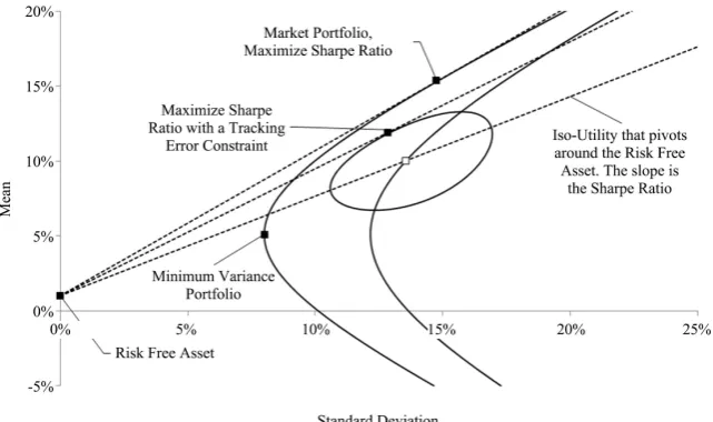
f

r . This ratio is simply the slope of a line connecting the risk free asset to any risky point in the Markowitz feasible set. See Figure 4 for representations of this line.

Maximizing the slope of this line in mean/variance space generates what is known as the Capital Market Line (CML) and its intersection with the minimum variance envelope is called the market portfolio.

[image:12.595.210.531.411.601.2]

The problem with the risk free asset in the context of a general solution to the variance minimization problem is that the covariance matrix, Ω, is no longer invertible because the risk free asset creates a row and column of zeros. Thus, Equation (2.1.1) is not a valid solution in this scenario. Finding the CML under the standard linear constraints of portfolio optimization is rather straight for-ward but with a general linear constraint, it becomes slightly more complicated.

(13)

Maximizing the Sharpe Ratio with a General Linear Constraint

Below is the solution to the Sharpe Ratio maximization problem. It is important to note that the solution to the following problem gives the weight vector for what is called the Market Portfolio if the constraints are the standard weight and return constraints. The statement of the problem is below:

(

)

1 2

maxS= ′ −rf s.t. ′ = .

′ w

w r

w E c wΩw

This formulation doesn’t lend itself well to quadratic programming, so in or-der to solve it we will use a well-known result called the mutual fund theorem, from Merton [2], or the two fund theorem. Essentially, a linear combination of any two portfolios on the efficient envelope also resides on the efficient envelope. Thus, the solution to the maximization problem above is a linear combination of any other two portfolios on the efficient set. Therefore, I will use two of the re-sults I already derived, w∗ the variance minimization solution, Equation (2.1.1),

and wU the utility maximization solution, Equation (2.2.1).

(

)

1

1 1

.

−

− −

∗ = ′ ′

w Ω E EΩ E c

(

)

1

(

)

1

)

1 1 1 1 1

.

− −

− _′ − _′ − _′ − _′ −

= + −

U

w Ω E EΩ E c Ω r E EΩ E EΩ r

And, their linear combination is below with weight x:

(

1 x

)

∗ x .

= − + U

w w w

For simplicity, I define a new weight vector wH,

(

)

(

1

)

1 1 − 1 _.

− − −

∗ ′ ′

= − = −

H U

w w w Ω r E EΩ E EΩ r

And, the weight vector, w, becomes:

. x

∗

= + H

w w w

Plugging this vector into our function for S yields:

(

)

1 2

2 . 2 f x r S x x ∗ ∗ ∗ ∗ ′ + ′ − = ′ − ′ + ′ H

H H H

w r w r

wΩw wΩw w Ωw

H

w is particularly convenient because it can be shown that

(

)

1

(

)

1

1 1 1 1

0.

− −

− − − −

∗

′ H = ′ ′ − ′ ′ =

wΩw c EΩ E EΩ r c EΩ E EΩ r

Thus, S becomes:

(

₂

)

1 2.

f x r S x ∗ ∗ ∗ ′ + ′ − = ′ + ′ H H H

w r w r

wΩw w Ωw

Now basic calculus can be applied to find the maximum with respect to x.

(

)

(

)

3/ 2

2 d 0. d f x r S x _x ∗ ∗ ∗ ∗ ∗ ′ ⋅ ′ − − ′ ⋅ ′ = − = ′ + ′

H H H

H H

w w w r w r w w

w w w w

Ω Ω

(14)

(

)

. f x r ∗ ∗ ∗ ′ ⋅ ′ = ′ ⋅ ′ − H H H

w r w w

w w w r

Ω Ω

Next, we need to calculate the expected returns and variances to reparametrize the expression into the proper variables and find the constant:

(

)

(

)

(

)

(

)

(

)

1 1

1 1 1

1 1

1 1 1 1

1 1 1 1 1 . f f x r r − − − − − − − − − − − − − − − − ′ − ′ ′ ′ ′ ′ = ⋅ ′ − ′ ′ ′ ′ ′ − ′ ′ = ′ ′ −

r r r E E E E r c E E c

r r r E E E E r c E E E r

c E E c

c E E E r

Ω Ω Ω Ω Ω

Ω

Ω Ω

And lastly, plug this constant back into the function for w=w_∗+xw_H:

(

)

(

)

(

)

(

)

(

)

1 1 1 1 1 1 1 1 1

1 1 1

. f r − − − − − − − − − − − −  _′ _′    ′ ′ = _{+ } _  ′ ′ −    ′ ′ ⋅ −

c E E c

w E E E c

c E E E r

r E E E E r

Ω Ω Ω

Ω Ω

Ω Ω Ω

(4.1.1)

Thus, this is the weight vector that maximizes the Sharpe Ratio given a general linear constraint, or equivalently, if the constraints are the standard Markowitz constraints, this is the weight vector of the market portfolio. It is expressed in the familiar and convenient form of a shift to the minimum variance weight vector.

5. Conclusions

In this paper, I derive the solutions to portfolio choice problems with a general linear constraint when they are also subject to a tracking error constraint. The primary method used to derive the solutions is quadratic programming. This essay connects the research of some of the most fundamental papers in the field of portfolio choice and generalizes a solution to the Tracking Error Volatility constraint problem of Jorion [8]. I set up the objective function in both variance minimization and utility maximization. Although Jorion solves the variance mi-nimization problem for specific constraints, my method solves the problem with a general constraint. Moreover, Jorion does not derive the utility maximization problem with a tracking error constraint, which I have done in the essay with a general linear constraint.

(15)

risk free rate is assumed to exist.

There are limitations to empirical research given these derivations. Real world data is oftentimes too volatile to apply the methods of modern portfolio theory directly. These derivations are best used as a conceptual framework to make theoretical assertions about the behavior of investment managers. The implica-tions from these theories can, however, be creatively tested and existing empiri-cal data can be used to discover nuances of the decision-making or real world investment managers. One example in particular that this model exposes is that managers that are incentivized by relative risk and return metrics will usually build portfolios that are riskier than a principal would desire. Although these equations likely couldn’t test that. This result could be tested in numerous other ways.

There are many other examples of constrained portfolio choice problems that fall into the framework outlined in this paper. Although my final expressions are cumbersome, they are also left in their purist form so the reader can see the form unobstructed by substitution. The general linear constraint is very useful when considering real world constraints to asset management, and the tracking error constraint is a pervasive, explicit and implicit constraint to which almost all asset managers abide. This paper will hopefully allow researchers to compare the ef-fects of differing constraints on portfolios in a more approachable manner, with the solutions readily available.

Conflicts of Interest

The author declares no conflicts of interest regarding the publication of this paper.

References

[1] Markowitz, H. (1952) Portfolio Selection. The Journal of Finance, 7, 77-91. https://doi.org/10.1111/j.1540-6261.1952.tb01525.x

[2] Merton, R.C. (1972) An Analytic Derivation of the Efficient Portfolio Frontier. Journal of Financial and Quantitative Analysis, 7, 1851-1872.

https://doi.org/10.2307/2329621

[3] Best, M.J. and Grauer, R.R. (1990) The Efficient Set Mathematics When Mean-Variance Problems Are Subject to General Linear Constraints. Journal of Economics and Business, 42, 105-120. https://doi.org/10.1016/0148-6195(90)90027-A

[4] Binsbergen, J., Brandt, M. and Koijen, R. (2008) Optimal Decentralized Investment Management. Journal of Finance, 63, 1849-1895.

https://doi.org/10.1111/j.1540-6261.2008.01376.x

[5] Blake, D.A., Rossi, G., Timmermann, A., Tonks, I. and Wermers, R. (2013) Decen-tralized Investment Management: Evidence from the Pension Fund Industry. The Journal of Finance, 68, 1133-1178. https://doi.org/10.1111/jofi.12024

[6] Cuoco, D. and Kaniel, R. (2011) Equilibrium Prices in the Presence of Delegated Portfolio Management. Journal of Financial Economics, 101, 264-296.

https://doi.org/10.1016/j.jfineco.2011.02.012

(16)

Portfo-DOI: 10.4236/jmf.2019.94034 690 Journal of Mathematical Finance lio Management, 18, 13-22. https://doi.org/10.3905/jpm.1992.701922

[8] Jorion, P. (2003) Portfolio Optimization with Tracking-Error Constraints. Financial Analysts Journal, 59, 70-82. https://doi.org/10.2469/faj.v59.n5.2565

[9] Bertrand, P. (2010) Another Look at Portfolio Optimization under Tracking Error Constraints. Financial Analysts Journal, 66, 78-90.

https://doi.org/10.2469/faj.v66.n3.2

[10] Chen, L., Peng, J., Zhang, B. and Rosyida, I. (2017) Diversified Models for Portfolio Selection Based on Uncertain Semivariance. International Journal of Systems Science, 48, 637-648. https://doi.org/10.1080/00207721.2016.1206985

[11] Kar, M.B., Kar, S., Guo, S., Li, X. and Majumder, S. (2019) A New Bi-Objective Fuzzy Portfolio Selection Model and Its Solution through Evolutionary Algorithms. Soft Computing, 23, 4367-4381. https://doi.org/10.1007/s00500-018-3094-0