School of Economics and Finance
Endogenous Infrastructure Development
and Spatial Takeoff
Alex Trew
Endogenous Infrastructure Development and
Spatial Takeoff in the First Industrial Revolution
∗
Alex Trew
†University of St. Andrews
January 17, 2019
Abstract
This paper develops a model in which the evolution of the transport sector occurs alongside the growth in trade and output of agricultural and manufacturing firms. Simulation output captures aspects of the historical record of England and Wales over 1710–1881. A number of counterfactuals demonstrate the role that the timing and spatial distribution of infrastructure development plays in determining the timing of takeoff. There can be a role for policy in acceler-ating takeoff through improving infrastructure, but the spatial distribution of that improvement matters.
JEL Classifications: H54; N13; N93; O11; O18; O33; R12.
Keywords: Industrial revolution, growth, transport, spatial development.
∗I am grateful to Leigh Shaw-Taylor for permission to work with the data produced by the Cambridge
Group. I thank two anonymous referees for comments that have greatly improved this paper as well as Dan Bogart, Mark Casson, Radek Stefanski and Scott Swisher for helpful discussion as well as seminar participants at Bristol, Cambridge, St. Andrews, Warwick and the 2017 DYNARE conference in Tokyo. I am grateful for support from the Institute for New Economic Thinking grant #INO15-00025.
†School of Economics and Finance, University of St. Andrews, St. Andrews, Fife, UK, KY16 9AJ. Tel:
1
Introduction
This paper studies infrastructure development in the context of a growth model where
trade occurs across a continuum of space (after Desmet and Rossi-Hansberg, 2014) and where the costs of trading across that space are a function of the endogenous supply of
in-frastructure at each location. By explicitly modelling the geography and the endogenous
determination of trade costs, we can capture the bi-directional interaction between the
evolution of trade costs and the location, concentration and growth of firms in different
sectors. Such interaction can happen via two channels. First, the growth of employment
in transport and distribution services can be a response to the growth of, and the spatial
concentration in, the agricultural and industrial sectors. Second, the demand for new
in-frastructure investment can emerge in different locations as some regions become wealthy
or as industrial hotspots emerge far from large markets for first-geography reasons. In turn, the employment of labour in transport services means less labour is available for
industry and agriculture; this may lower firm scale and delay the onset of investment in
innovation. Further, the lower transport costs that follow infrastructure improvements
stimulate further changes to the economic geography. With the model in hand, we match
quantitative aspects of the macroeconomic and spatial history of England and Wales over
the period of the industrial revolution, from 1710 to 1881. We then use counterfactual
treatments of the model to consider the dynamic impact on growth of policies that change
the timing and spatial distribution of infrastructural development.
Investment in transport infrastructure is often central to efforts at stimulating
devel-opment in low-income countries (World Bank, 2015). We know that significant change in economic geography is a feature of development (Desmet and Henderson, 2015) and
that falling transport costs have an impact on economic activity (Redding and Turner,
2015). We have only a limited understanding, however, of how transport costs, economic
geography and economic growth interact in an economy going through a transition to
high growth. How does the quantity of labour employed in the tertiary sector, the
quan-tity of infrastructure investment, its timing relative to transition to high growth, and its
geographical focus, affect long-run macroeconomic outcomes such as structural
transfor-mation and the emergence of sustained high growth? The answers to these questions
should inform policies directed toward infrastructure.
Modern infrastructure investment, even if financed in partnership with the private
sector, is generally organized and planned by the State. The experience of England and
Wales during the industrial revolution, in contrast, was of infrastructure development that
was largely driven locally by private enterprise. The industrial revolution was
accompa-nied by a revolution in transport infrastructure that occupied an increasing proportion of
the workforce and that vastly reduced the cost and increased the speed of transporting
goods (Bogart, 2014). That transport revolution was a response to, and stimulant of,
the 18th and 19th centuries. England and Wales thus provides a useful benchmark
en-vironment in which we can understand the development of transport infrastructure in
a laissez faire economy. With a model of that infrastructure development in hand, we
can conduct counterfactual analysis to explore the consequences of an alternative
infras-tructure policy, such as ones similar to those seen today. While we may be hesitant to
compare early industrial England and Wales to the modern world, there are Continental European examples in this historical period where centralized infrastructure policy
sig-nificantly affected the timing and spatial distribution of transport developments (Smith,
1990). Among others, Szostak (1991) has made the case that those policies also delayed
growth. Although there are significant differences today, such as the rise of commuting,
modern infrastructure is subject to many of the same underlying changes in demand that
emerge endogenously as spatial economic change occurs. By studying whether historical
policies that centralise infrastructure development had real consequences, we can thus
begin to learn about how infrastructure policy and growth are fundamentally related.
We develop a model that captures the evolution of the transport sector in England and Wales over the period 1710–1881. To do so, we introduce endogenous transportation
costs to the framework of spatial development in Desmet and Rossi-Hansberg (2014).
In particular, we make the cost of transporting goods through a location endogenous to
the supply of infrastructure at that location. Infrastructure supply is part stock of fixed
infrastructure and part transportation service produced by local carriers.
Landowner-carriers1 hire transportation labour to facilitate the wholesaling and distribution of goods
through their land. Landowners may also lease land to infrastructure companies who
improve the infrastructure on their land. As in Desmet and Rossi-Hansberg (2014), firms
can invest in developing improved production methods at a location and, as in Trew (2014), non-homothetic preferences mean that consumption shifts toward manufactured
goods as incomes grow. The evolution of the transport sector occurs simultaneously with
those firm decisions that drive the aggregate takeoff in growth rates and the structural
transformation of the economy.
We initialize the model using data for the occupational structure of England and
Wales at 1710. We then run the model for 171 periods and track its predictions against
various macroeconomic variables, such as average growth rate and overall structural
trans-formation, as well as against the spatial distribution of employment in each sector, the
endogenous decline in transport costs and the spatial distribution of infrastructure im-provements. An industrial takeoff in the North of England, and the specialization of the
South in agriculture, means that a greater quantity of output is traded over greater
aver-age distances. The demand for transportation improvements emerges locally as a response
to the demand for inter-regional trade. Since transport costs also affect the scale of
pro-1While agents in the model own a diversified portfolio of all land, we refer to ‘local landowners’ as
duction, incentives to innovate and the emergence of agglomerations, there is a feedback
from that infrastructural development to the speed of the takeoff in growth.
By modelling infrastructural development as an endogenous process, and by matching
that model to the historical experience during the industrial revolution, we can ask how
policies which depart from the experience in England and Wales may have affected the
timing and speed of takeoff. We find that the timing and spatial distribution of infrastruc-ture improvements can matter. In particular, we show that exogenously higher transport
costs can bring forward the date of takeoff as it increases the agglomeration forces that
make it more likely firms overcome the fixed costs of innovation. However, early
infras-tructure investment can accelerate industrial takeoff since it also releases labour out of
providing transportation services. Large gains from early infrastructure are only realized
if the infrastructure investment is focused on those locations that have a local demand
for it. If an equivalent infrastructure improvement is implemented in a spatially-uniform
way, the impact on the timing of takeoff is severely muted.
1.1
Related Literature
The paper builds on a number of different strands in the literature. First, we relate to the literature on urban economics, development and the impact of trade costs. Desmet
and Henderson (2015) surveys the literature on the relationship between economic
devel-opment and the changing geographical organization of economic activity. As they show,
one particular avenue for research is in modelling the interplay between macroeconomic
outcomes, such as growth, and the spatial distribution of economic activity. For this
paper, technological progress occurs as firms attain scale in cities; those agglomerations
are themselves a function of a transportation network that evolves as the economy grows.
While there is a recent literature2 that makes endogenous the costs of transportation, or the transport network itself, these are limited to static models and, mostly, a discrete number of large spatial units. Here, we study trade across a continuum of space and
adopt the spatial development framework of Desmet and Rossi-Hansberg (2014). A
fur-ther contribution is in understanding the role of transport costs on economic activity.
Redding and Turner (2015) surveys the literature that looks to identify the consequences
of exogenous variations in infrastructure supply on the spatial distribution of economic
activity. These include structural approaches such as Donaldson (2015) and Allen and
Arkolakis (2014). Those papers incorporate the general equilibrium effect of improving
market access in one location on activity in other locations. Such models tend, again, to
be static and typically only model one sector (agriculture). Nagy (2015) models spatial
development over time in two sectors and obtains results on the impact of infrastructure on growth. Here we model structural transformation and evolution of infrastructure as it
occurs over one-dimensional space and time. Fajgelbaum and Schaal (2017) studies the
optimal design of infrastructure networks, but in a static model.
Second, the paper relates to the literature on growth, structural transformation and
transport costs. As shown in Desmet and Rossi-Hansberg (2012), one way to generate
endogenous growth is to model firms that innovate based on it being tied the use of land
as an excludable factor of production. This paper uses that framework and extends Trew (2014) to incorporate labour employed in the transport sector. It thus contributes to
the literature on structural transformation (see Herrendorf et al., 2014). A number of
papers, such as Adamopoulos (2011), Herrendorf et al. (2012) and Gollin and Rogerson
(2014), show how exogenous transport costs affect labour allocations in a static setup
with exogenous growth. For this paper, transport costs and growth evolve endogenously
over time.
Third, we contribute to the literature on the industrial revolution. Shaw-Taylor and
Wrigley (2014) have recently shown that the truly dynamic part of the economy over the
course of the 19th century, the period in which per capita growth took off (Crafts and Harley, 1992), was the tertiary sector. A large portion of that tertiary sector growth
constituted a transport revolution that was projected by largely private enterprise which faced a need to reduce the costs of inter-regional trade (Bogart, 2014). Szostak (1991) is
among those that have made a case for the importance of transportation Britain’s early
industrial lead over France. Recent work by Desmet et al. (2015) investigates how lower
transport costs increased spatial competition, reduced the power of guilds and led to
industrialization. This paper contributes to that debate by simultaneously modelling the
role of transportation services and growth. By conducting counterfactual exercises, we
can ask whether industrial takeoff may indeed have been delayed as a result of different transport policies.
1.2
Outline
In Section 2 we briefly discuss England and Wales during the industrial revolution as well
as evidence on the nature of the transport revolution during that time. We develop the
full model of endogenous infrastructure in two steps. First, in Section 3 we make labour
in transport and distribution endogenous to output and trade across space but keep the
infrastructure stock fixed. In Section 4 we present simulation results which demonstrate
that this model can match the aggregate and spatial development of England and Wales
over the period 1710–1881. Second, in Section 5 we extend the model to allow endogenous
investments in infrastructure stock, comparing the model to the data for England and
2
Occupational change, growth and transportation
in England and Wales, 1710–1881
We focus on the industrial revolution in England and Wales for two main reasons. First,
infrastructure development in England and Wales during the 18th and 19th centuries
was relatively decentralized (see Trew, 2010). Today, infrastructure projects are
care-fully planned by central governments (even where financed privately). For 18th and 19th
century England and Wales, infrastructure development was characterized by local
pro-jection (i.e., not organized into a national system) and local finance. While the contrast
to modern policies is clear, we can, as discussed below, draw a more direct historical
contrast in the policies toward infrastructure between Britain and France. Second, we
have exceptionally detailed data at high spatial resolution for England and Wales over
the period when it was the first nation to enter a sustained period of high growth and the scene of the most rapid revolution in the speed and cost of transportation to that
date. This data permits an understanding of the changing economic geography and
spa-tial takeoff that underpinned the industrial revolution. We can thus ask whether and how
the development of infrastructure interacted with the spatial takeoff.
2.1
Occupational structure and growth
For occupational information we use the data described in Shaw-Taylor et al. (2010a) at
three dates: 1710, 1817 and 1881. The data is observed at the level of 624 registrations
districts covering nearly all of England and Wales. For 1881, the available census records
provide a complete picture of the local occupational structure. For 1817, there was no
such occupational census. Shaw-Taylor et al. describe the process of constructing a ‘quasi-census’ based on information in parish baptismal records. The data for 1710 uses
the observations of baptismal records in 1,062 of the 11,102 ancient parishes in England
at that time. Trew (2014) uses this sample to construct predicted values for the number
of adult males in each major occupation (primary, secondary, tertiary and textiles) at the
level of the registration district.
Occupations are categorised using the Wrigley (2010) Primary-Secondary-Tertiary
(PST) system. Primary occupations are mainly agriculture but also forestry, fisheries
and mining (the latter of which we remove).3 Secondary occupations are manufacturing, processing and construction. The tertiary sector is composed of four groups: Transporta-tion and communicaTransporta-tion; sellers; dealers; and professionals. The distributive sector (i.e.,
the tertiary sector less professions) makes up over half the total tertiary employment
3In the Wrigley classification, the Primary sector includes mining. We remove mining since it behaves
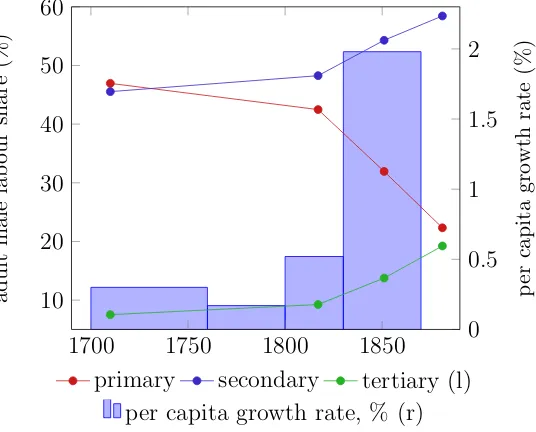
through the period of study. We use the tertiary sector without professionals.4 Figure
1 depicts the aggregate structural transformation at the PST level, with professions and
mining omitted, alongside the trend in per capita growth of output over the same period
[image:8.595.167.435.178.394.2]from Mokyr (2004).
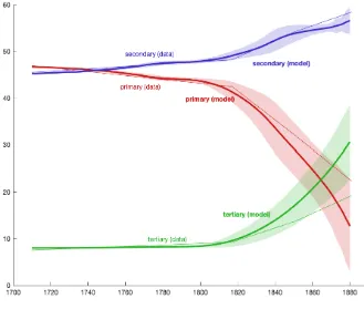
Figure 1: Occupational structure and growth
0 0.5 1 1.5 2 p er capita gro wth rate (%)
per capita growth rate, % (r) 1700 1750 1800 1850 10 20 30 40 50 60 adult male lab our share (%)
primary secondary tertiary (l)
Figure 1 captures the surprising aspect of the Shaw-Taylor et al. (2010b) findings (see
also Shaw-Taylor and Wrigley, 2014). The secondary sector is stable and growing over the
course of the 18th and 19th centuries, from 45% in 1710 to 48% in 1817 and finally 58%
in 1881.5 The decline in the primary sector starting early in the 18th century accelerates
after 1817 but this is not reflected entirely by a growth in the relative importance of
industry. Instead, the decline in agriculture is accompanied by the rapid growth of the
tertiary sector. Most strikingly, the accelerated shift of labour out of the primary sector
and the rapid increase in the tertiary sector is coincident with the takeoff in per capita
growth. At a macroeconomic level, this suggests that there is something missing in the typical understanding of growth as simply a result of a shift of resources from agriculture
to industry alone. One way of understanding this is bound up in space, as Shaw-Taylor
et al. (2010b) conjecture:
It may be that the majority of tertiary growth in the 19th century was required simply to move the greatly increased output of primary and secondary goods
longer average distances around the country. If this is the case then the rise
of the tertiary sector was caused, at least in part, by the marked expansion in
4The trend for tertiary including professions and services over the 19th century is much like that shown
in Figure 1. When we refer to tertiary employment in this paper, we mean tertiary less professionals.
the productivity of other sectors and in that sense heralds the onset of modern
economic growth.
Shaw-Taylor et al. (2010b), p.21.
That is, tertiary employment growth can be a function of changes in the size and
spatial concentration of the primary and secondary sectors.
2.2
The spatial transformation
Economic activity is unevenly distributed across space and that unevenness can change
over time and in different ways in different sectors. This is a form of spatial structural
transformation. If each sector changed uniformly at all points in space, or if each sector
each grew only at one point in space, then the complexity added by modelling that space
is not necessarily important for developing a model of what drives growth.
Since we have information at the level of the registration district, we can consider
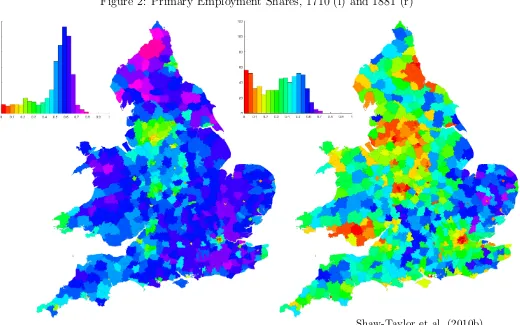
whether there was such a spatial structural transformation. Figures 2–4 use the
Shaw-Taylor et al. (2010b) data to map the registration district shares of adult male employment
in primary, secondary and tertiary occupations, respectively (colors represent share
lev-els6). The primary sector becomes more spatially specialized in the South and East of
England. The spatial distribution of the secondary sector is relatively stable over the
period. The small industrial hotspots are visible in the North and Midlands; these
be-come slightly larger over the period. As will be seen below, a significant characteristic
of change in the secondary sector results from movement of population to the industrial regions. Since, in local terms, those regions at the heart of the industrial revolution were
already highly industrialized at 1710, Figure 3 masks this important feature of spatial
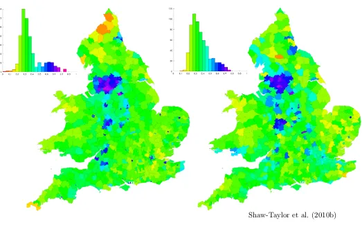
change. The most striking change is that shown in Figure 4. In particular, there is little
clear change to the spatial distribution of tertiary employment. Most areas outside the
London area have less than 10% of workers employed in the tertiary sector at 1710. By
1881, no registration district has less than 5% employed and the modal share is in the
10-15% range. The growth in the local importance of the tertiary sector occurs uniformly
across all areas of the country, whether they were initially agricultural or industrial. The
growth in shares of tertiary employment thus means that in absolute terms, tertiary em-ployment grows along with the growth in emem-ployment in other sectors.
The spatial structural transformation in England and Wales over the period 1710 thus
takes the form of a primary sector that declines in the North and grows in the South, a
secondary sector that maintains its Northern hotspot and a tertiary sector that grows in
relative importance at most points in space. A model of this spatial detail, and of how
6The histograms at the North-West of each panel are the count of registration districts (y-axis) against
different sectors change spatially over time, could be necessary to understand the drivers
[image:10.595.42.562.103.428.2]of takeoff in the first Industrial Revolution.
Figure 2: Primary Employment Shares, 1710 (l) and 1881 (r)
Shaw-Taylor et al. (2010b)
2.3
The transport revolution
Alongside the changes to the number of workers employed in the tertiary sector is
signifi-cant investment in infrastructure capital and declines in the costs of transportation. The
nature of the transport revolution in Britain is discussed in Bagwell (1974) and the
excel-lent survey in Bogart (2014). For Bagwell (p.15), “It was the rapidly increasing volume
of inter-regional exchange that made imperative the introduction of more sophisticated
forms of goods transport.” Those improvements took the form of new technologies such
as better paving and river improvements, as well as better modes of transport. For the purposes of this paper, we treat the improvements within a mode and across modes of
transport as one continual improvement in transport infrastructure.
The principal means of improving inland transportation in the early 18th century was
the introduction of privately managed roads in the form of turnpike trusts. These trusts,
while not profit-making, were permitted by Act of Parliament to charge tolls for passage
along the road. As Buchanan (1986) and Bogart (2007) describe, the trusts were run by
Figure 3: Secondary Employment Shares, 1710 (l) and 1881 (r)
[image:11.595.44.561.436.730.2]Shaw-Taylor et al. (2010b)
Figure 4: Tertiary Employment Shares, 1710 (l) and 1881 (r)
distinction is also apparent between the role of the funds raised for the initial turnpike
improvement and the levying of tolls for subsequent current spending on maintenance.7
The second major mode of transport took the form of extending navigable rivers and
the construction of canals, particularly from the early 19th century on. For canals,
Par-liament authorized the formation of joint-stock companies that could raise the capital
required for the expected construction costs. Using data on subscriptions to canal com-pany stock, Ward (1974) shows that, as with turnpikes, the canals were organized and
financed by those local to the infrastructure. By consequence, as Turnbull (1987) finds,
those early canal improvements again served local markets in a way that was not
ini-tially connected to a national system. As Hadfield (1981) describes, canal companies did
not typically also provide carrier services to those wishing to move freight (until 1845
they were not permitted to do so without an Act of Parliament). Into the 19th century,
the construction of railways became the means of improvement to inland transportation.
Once more, as Hunt (1935), Broadbridge (1955) and Shea (2012) document, the railways
were often projected for local purposes on the back of local subscriptions to the railway companies. Broadbridge (1955) finds that ‘local interests’ in financing railways remained
dominant until the latter half of the 19th century.
The formation of an infrastructure company was thus the vehicle to overcome the fixed
costs of an improvement with the aim to increase the value of local land and the profits
of local businesses. Subsequent tolls were typically for maintenance of the infrastructure
and for carriage of goods on that infrastructure which was, particularly for roads and
waterways, typically carried out by separate entities. Given the uncertainties of the new
technologies and unknown local demand, the opportunities for speculation by remote
investors were limited and, where investment mania occurred, schemes began to reserve shares for landowners on the route and for the inhabitants of local towns (Pollins, 1954). In
many cases, the companies were explicitly promoted as being in the local public interest.8
An infrastructure company was thus a concern which improved the local economy first,
and provided returns to the company shareholder second.
One further aspect of the history worth noting is the nature of dispute resolution when
alternative proposed routes were in conflict. Since an Act of Parliament was needed to
approve the formation of a trust or joint stock company, competing interests benefited
from submitting a single proposal to Parliament with support from those Members of
Par-liament that owned the land along the route. ParPar-liament was typically not the venue for conflict; as Harris (2000, p.135) notes, it “served only as the arena and set the procedural
rules.” As such, many non-controversial projects were approved in Parliament with little
7As Buchanan (1986, p.228) notes, the Acts of Parliament allowed the “raising of funds in a financial
market and the levying of tolls on road users... in general the former provided the long-term capital of the Trust (invested in new and improved roads with their attendant Parliamentary and legal costs) and the latter its current revenue (spent on road repairs, administration, and interest payments)”.
8The motto of the Trent & Mersey Canal, completed in 1777, wasPro Patriam Populumque Fluit –
conflict. In some instances, however, neighboring cities and counties disagreed on the
route to be taken by a canal or railway that would connect them. A good example of the
resolution of competing projects is the Leeds and Liverpool Canal, which was authorized
in 1770 (see Clarke, 1994). Manufacturers in Yorkshire wanted access to Atlantic trade
and a supply of lime for improving agricultural land, while those in Lancashire needed
access to the coal inland. Committees in both Yorkshire and Lancashire were formed and as many as five different routes were proposed. A solution was sought by the employment
of an arbitrator who chose a route based on the interests of both counties. As Clarke
(1994, p.68) concludes, “Following the solution of various disagreements... progress of the
Bill through Parliament was swift.” The resolution of competing railway plans was often
less straightforward, with much debate within Parliament. As Bagwell (1974, p.101)
de-scribes, the main consequence was “a golden harvest” for the solicitors representing each
interest to Parliament. The sum spent on securing Parliamentary authorization was
lim-ited to only two per cent of total outlay on railway capital, at the end of which Parliament
would reconcile competing interests and authorize a single company.
The pattern of local projection and local finance of transport improvements reveals
just how endogenous the transport network was to regional economic developments. Since
industrial developments occurred in a small number of hotspots, thus did infrastructure
improve alongside those local developments. Those producers wishing to transport their
goods faced two costs: First, the infrastructure company charged a toll on the users of the
turnpike, canal or railway. Second, the carrier (the owner of the wagon or boat) charged
a fee based on the quantity and type of goods to be carried as well as the distance to
be travelled. The overall fall in transport costs over the period was dramatic. Bogart
(2014) collates data (see Figure 5) that demonstrates there was a 95% reduction in real shillings per ton mile from 1700 to 1865 across all forms of transport (road, waterway,
rail). The fall in freight cost between waterways in 1730 to rail in 1865 is 86%. It should be
noted that this is a na¨ıve estimate of the decline in transport costs. The declining freight
charges for a growing canal and railway network may be partially offset by the increasing
need to move goods across different parts of an increasingly multi-modal network. Recent
evidence in Alvarez-Palau (2018) on the costs of trans-shipment across roads, coasts and
canals up to 1830 suggests that 15% of freight costs can be attributed to trans-shipment.
As the railways later emerged, adding a dimension to trans-shipment costs, real freight
charges would be even higher by the end of our period.
To put British infrastructural development into an historical contrast, we can compare
it with the situation in France and Germany. The Becquet plan of 1822 envisioned a
public-private partnership: A centrally planned waterway system paid for by private
capital. A group of civil engineers, the Corps des Ponts et Chauss´ees, was charged with
setting and enforcing the regulations for a waterway network of sufficient quality. As L´
Figure 5: Freight costs (Bogart, 2014)
1700 1750 1800 1850 0
0.2 0.4 0.6 0.8 1 1.2
shillings
p
er
ton
mile
(1700
prices)
road waterway rail
extended beyond canals and covered also railways. At their introduction, there was also
uncertainty over the role of railways in the context of the canal plan (Smith, 1990).
Even once Napoleon III began to promote the private finance of a dominant railway
infrastructure, private plans were still subject to the layout, location and specifications dictated by the Corps. Milward and Saul (1973, p. 336) argue that government “beset
railway building with so many safeguards as to delay its flourishing by a full decade.”
In contrast to France, disunity of German states meant that no such co-ordinated plan
could be developed. As Smith (1990) notes in regard to Germany, a liberal railroad law
emerged in 1838 “left companies the intiative to propose routes as well as engineering
design” (p.671).
3
Model with exogenous fixed infrastructure
We briefly outline the structure of the model before developing it in detail. Trew (2014)
introduces non-homethetic preferences into the spatial development framework of Desmet
and Rossi-Hansberg (2014, henceforth DR-H). In this set-up, we have two final goods:
Agricultural and manufacturing. As income grows, the marginal utility from consuming
agricultural (manufacturing) goods declines (increases) and so consumption (and labour
demand by firms) shifts towards manufactured goods. Firms, arranged along an interval
of space, hire labour and rent land; they can also invest in a chance to improve their
production technology.9 Perfectly mobile workers can move in advance of productivity
9To establish the importance of modelling with a continuum of locations, we introduce in Appendix
realisation to the location that yields the greatest expected utility. Subsequent to
inno-vation and production, there is spatial diffusion of productivity before the start of next
period.
Since workers consume at the location of their employment, each point in space may
export one type of final good and import another. Such trade is costly and, in DR-H
and Trew (2014), this cost is assumed to be a fixed iceberg cost. This present study is of the development of transport infrastructure so we make additional departures from
Trew (2014) as motivated by two facts. First, at an aggregate level, Section 2 showed
that a substantial portion of labour is employed in the tertiary sector (that is, without
professionals: transport, distribution and wholesaling). Second, significant resources are
expended on improving the stock of infrastructure at a location by, for example, improving
roads or constructing canals. Transport costs at a location are determined by both the
labour employed in transport and wholesaling and by the stock of transport infrastructure
at a location. Moreover, both the labour employed and the stock of infrastructure varies
significantly across space and changes over time.
In this section, we make transport costs endogenous to the infrastructure supply at
each location. Infrastructure supply is part stock of fixed infrastructure, which we initially
take to be exogenous, and part labour used to facilitate the transportation of goods
through a location. Conditions on the equilibrium relationship between infrastructure
stock, transport labour and transport costs for equilibrium are identified. In particular,
while equilibrium trade determines the demand for labour in transport, that labour in
transport is also drawing labour away from the production of final goods. As such, we
need to ensure that an equilibrium in the goods and labour markets exists. We consider
the quantitative performance of the model against the data in Section 4. In Section 5, we make the supply of fixed infrastructure over connected intervals endogenous to investments
by infrastructure companies in those intervals.
3.1
Preferences
Agents earn a wage w(`, t) from supplying labour to firms which are ordered at points `
on the closed interval of land [0,1], as in DR-H. Agents also hold a diversified portfolio
of all land and so receive an equal share of all rental income, R(t)/L¯ where R(t) is the
aggregate land rent and ¯L is the fixed total labour supply. There is no storage good. A
consumer solves the following optimization problem,
max
{cA(`,t),cM(`,t)}∞0 E
∞ X
t=0
βtU(cA(`, t), cM(`, t)) (1)
s.t. w(`, t) + R(¯t)
L =pA(`, t)cA(`, t) +pM(`, t)cM(`, t), ∀(`, t),
where cA(`, t) and cM(`, t) is consumption of agricultural and manufacturing goods,
re-spectively,pA(`, t) andpA(`, t) are prices of agricultural and manufacturing goods,
respec-tively, andU(·) is the instantaneous utility function that takes the following Stone-Geary
form, as in Trew (2014),
U(cA(`, t), cM(`, t)) = (cA(`, t)−γ)η(cM(`, t))1−η (2)
where η∈ (0,1) and γ >0 captures a subsistence requirement in agriculture. Given free mobility of labour, equilibrium prices, wages and rental income equalize utility to ¯uacross
all locations at a given point in time.
3.2
Firms and innovation
A firm at location` can produce either agricultural or manufacturing goods using labour
Li(`, t) and productive land10 (which is normalized to one),
A(`, t) =ZA(`, t)LA(`, t)α, (3)
M(`, t) =ZM(`, t)LM(`, t)µ, (4)
where α < µ captures agricultural production that is more land intensive and where
ZA(`, t) and ZM(`, t) are the location-dependent productivity levels in each sector.
Prior to hiring labour and making a bid for land, firms may expend resources on
obtaining a draw for better technology at their location. In particular, a firm buys a probability φ of innovating at sector-dependent cost ψi(φ). If a firm is successful in
innovating, it draws a ˆz from a Pareto distribution with minimum value 1 and Pareto
parameter ai.11 Successful innovation yields a production technology of ˆzZi(`, t). We let
the expected draw be greater in manufacturing than in agriculture (i.e., aA > aM). The
expected technology for a firm that spends resources on a chance at innovation is thus,
E(Zi(`, t)|Zi) =
φ ai−1
+ 1
Zi. (5)
Firms that attempt to innovate may offer a greater rent to landowners if the expected
gains from innovating outweigh the costs. However, at the end of each period (after
production and consumption), technology in each sector is spatially diffused with decay
10Each location can hold transport infrastructure on unproductive land.
11We assume that innovation draws are spatially correlated – firms arbitrarily close receive the same
δ, that is,
Zi(`, t) = max
r∈[0,1]e
−δ|`−r|
Zi(r, t−1). (6)
Since labour is perfectly mobile, and since technology diffuses at the end of each
period, DR-H show that despite the persistence of the new technologies that emerge from innovation, the advantage to innovators dissipates leaving the firm problem as a
maximization of current-period profits. That is, a firm chooses φi to solve,
max
φi
pi(`, t)
φ ai−1
+ 1
ZiLˆi(`, t)ı−w(`, t) ˆLi(`, t)−Rˆi(`, t)−ψ(φ(`, t)), (7)
There are fixed and marginal costs to obtaining a chance of innovation. As in Trew
(2014), we let these costs vary by sector and, in particular, we account for the feature of
industrial growth that innovative manufacturing technologies were more energy-intensive than agricultural ones. The cost of drawing a probability of innovation φ in sector i is,
ψi(φ) = ψ1,i+ Γiξ(`) +ψ2,i
1 1−φ
if φ >0, (8)
whereξ(`) is the energy cost at location `,12 ψ1,i >0 is the fixed cost parameter, ψ2,i >0
is the marginal cost parameter and Γi = 1 ifi=M and 0 otherwise.13 Conditional on the
expected net gain being positive, firms choose the φthat maximize the expected increase in net profits, that is, the optimal investment probability is,
φ∗i(`, t) = 1− ψ2,i(ai−1)
pi(`, t)Zi(`, t) ˆLi(`, t)ı
!1/2
. (9)
As can be seen from equation (9), there is a scale effect present in the intensity of
in-novation: Higher output at a location is accompanied by a higher optimal innovation
probability.
3.3
Transport costs and tertiary labor
Transport infrastructure at a location is composed of a fixed infrastructure (roads, canals, railway tracks) and a transportation service (which would include carriage services, rolling
stock, and so on). We assume that the fixed infrastructure is free to access and exogenously
fixed until Section 5. In this section, we introduce the role of a landowner-carrier that
12We choose this form of energy costs as an alternative to introducing a second secondary production
technology since we do not have data to initialize the model with seperate energy-intensive secondary and traditional secondary sectors. In practice, once a firm begins to find it optimal to draw an innovation it continues to do so in each period thereafter (thus generating the sustained growth observed in simulations below).
13As in DR-H, in simulations we makeψ(·) proportional to wages to ensure that the cost of innovation
provides transportation services. The carrier charges a toll for the carrying of freight and
the construction of rolling stock to run on the fixed infrastructure. We assume that the
rolling stock fully depreciates each period. While full depreciation is a simplification, the
difference between the longevity of the fixed infrastructure and rolling stock is clear in
England and Wales, as elsewhere, where new trains can run on Victorian tracks and where
new lorries drive on decades-old roads.
Both the fixed infrastructure and the transportation service determine the cost of
transporting goods through a location. The transport cost is made up of a physical cost,
¯
κ(`, t), and a toll, ˜κ(`, t), charged by landowner-carriers. The total transport cost is,
κ(`, t) = ¯κ(`, t) + ˜κ(`, t). (10)
The physical cost results directly from the level of the local fixed infrastructure stock,
T(`, t). Improving fixed infrastructure reduces the cost of transporting goods by, for
example, increasing the speed of travel or by increasing the quality of transportation
(reducing spoilage, spillage, and so on). This physical cost is akin to a standard ‘iceberg’
cost and is lost to the economy. However, the toll is charged by a landowner to fund the
production of the transportation service and is paid to transportation workers who then
use that income to consume goods. Since the toll ˜κ(`, t) is not lost to the economy in a
normal iceberg-sense, the price of a good i being shipped from locations to location r is
thus a function of the physical cost alone,
pi(r, t) = exp
Z r
s
¯
κ(`, t)d`
pi(s, t). (11)
That is, the price of good shipped from location s to location r takes account of the
accumulated melt of the shipped good,Rsr¯κ(`, t)d`. In DR-H, the iceberg cost is assumed
to be fixed and labor is used only in the production of consumption goods, so ¯κ(`, t) =κ
and equation (11) reduces to pi(r, t) = eκ|r−s|pi(s, t).
In this paper, both parts of the transport cost are endogenous. We take the physical
transport cost ¯κ(`, t) to be a decreasing function of the fixed infrastructure stock, T(`, t),
¯
κ(`, t) =κe−T(`,t), (12)
where κ>0. In other words, a better infrastructure stock means faster (or more secure)
transport and less melt of goods. Since infrastructure is built on unproductive land at
each location, a higher T(`, t) does not reduce the land available at that location for firms.14 We keep T(`, t) fixed until Section 5.
14At peak, there were 35,684km of turnpikes in 1838, 9,069 km of navigable waterway in 1848 and
The toll is determined by a landowner who produces a transportation service to
trans-port goods using a CES production technology YT that is a function of an economy-wide
transport efficiency,ZT(t), transport labour hired,LT(`, t), and the local fixed
infrastruc-ture,
YT(`, t) =ZT(t) [ζLT(`, t)r+ (1−ζ)T(`, t)r]
1
r . (13)
where ZT(t) is exogenous but can grow over time. Production is characterized by a
constant elasticity of substitution betweenLT andT and we assume that transport labour
and fixed infrastructure are substitutes, r ∈ (0,1). An individual landowner takes the
fixed infrastructure as given, choosing labour LT(`, t) to maximize its return,
πT(`, t) = ˜κ(`, t)YT(`, t)−LT(`, t)w(`, t). (14)
For a given toll, the optimal choice of transport labour, ˆLT(`, t), taking ZT, T, and w as
exogenous, is,
ˆ
LT(`, t) =
("
w(`, t) ˜
κ(`, t)ZT(t)ζ
1−rr
−ζ
#
/(1−ζ)
)−1
r
T(`, t) (15)
Local labour employed in transport is, ceteris paribus, increasing in transport productiv-ity, infrastructure stock and the toll, decreasing in the local wage rate.
The demand for transportation services, D(`, t), is the sum of output produced at
a location (which requires wholesaling and distribution) and that traded through the
location (which requires transportation). The trade flow arriving at a location is taken
as given by its individual landowner. Since firms use a fixed amount of land and choose
labour and technology investment optimally subject to wages and prices, the output of
a given sector at a location is also invariant to the rent charged. As such, an individual
landowner takes this demand for transportation services to be exogenous. The toll that
satisfies demand, using YT(`, t) = D(`, t) and equations (13) and (15), is,
ˆ
κ(`, t) = w(`, t)
ZT(t)ζ
(
ζ(1−ζ)
D(`, t)
ZT(t)T(`, t)
r
−1
−1
+ζ
)r−r1
. (16)
Equation (16) is the minimum toll a landowner must charge to hire the transport labour
required to produce the output to meet the demand at their location. The minimum toll
is increasing in the demand for transportation services and so, by equation (15), is the
local demand for transport labour. For a given level of demand, the toll is decreasing in
ZT and T, increasing in w.
Since land is modelled as an interval, we assume that all locations between two points
r and s must be traversed. Any landowner between r and s could thus choose to set
˜
κ(`, t) = 1 to seize all trade flow for local consumption. In a two-dimensional reality, a
landowner that did so would find that trade flows around their location by an indirect
route over land or by shipping by sea along the coast. For the purposes of this model, we
suppose that at each location there is an indirect shipping technology that is identical to
equation (13) but has efficiency ˘ZT(t) = (1−ε)ZT(t). We may think of this lower efficiency
as resulting from the loading of goods onto and off of vessels that would otherwise would go through a location. By (16), this alternative implies a higher minimum toll at each
location and so ε captures the technological cost of shipping indirectly. This limits a
landowners rent from being the monopoly provider of transportation services at their
location. For simplicity we let this ε become negligibly small. Lemma 1 establishes the
choice of toll and conditions for it to be bounded.
Lemma 1 (i) The toll, κ˜(`, t), approaches equation (16) as ε → 0 in the presence of indirect shipping. (ii) κˆ(`, t)∈(0,1) if D(`, t)> ZT(t)T(`, t) and w(`, t) < ZT(t)ζ1/r for
all t and `.
Proof. (i) Indirect shipping around location ` with efficiency ˘ZT(t) implies a minimum
toll ˘κ(`, t) > ˆκ(`, t) at each location. If a landowner charges more than the
alterna-tive shipping then consumption at each location is constrained to that produced locally.
Since each location specializes in one sector, worker utility would be zero at any
lo-cation not engaging in trade. As a result, a landowner sets ˜κ(`, t) = ˘κ(`, t) and as
limε→0κ˘(`, t) = ˆκ(`, t). (ii) That ˆκ(`, t) > 0 if D(`, t) > ZT(t)T(`, t) follows from
equa-tion (13); if demand for transportaequa-tion services can be satisfied without transport labour
then the toll is zero. If D(`, t)/[ZT(t)T(`, t)] grows over time, (16) makes clear that
limt→∞κˆ(`, t) =w(`, t)/[ZT(t)ζ1/r].
With the toll determined by (16), transport labour is simply,
ˆ
LT =
D(`, t)
ZT(`, t)T(`, t)
r
−1
/ζ
1/r
T(`, t). (17)
Equations (15) and (16) capture two forms of congestion since higher transport demand generates a higher toll and greater tertiary labour. A higher toll lessens the increase in
trade and the greater transport labour increases local consumption of the final goods. As
such, we require that an increase in output at a location is not fully absorbed by a higher
toll or by higher local consumption of the extra tertiary labour. The same is true of an
increase in trade that results from higher output. The requirement that congestion is
not overwhelming places a slightly stronger restriction on the level of demand relative to
non-labour transport input, as the following Lemma shows.
Lemma 2 A sufficient condition for a limited congestion effect on the toll ∂D∂κˆ < 1 is
Proof. From equation (16),
∂κˆ(`, t)
∂D(`, t) =
(a)
z }| {
w(`, t)
ZT(t)ζ
(1−r)(ζ(1−ζ))
(b)
z }| {
(
ζ(1−ζ)
D(`, t)
ZT(t)T(`, t)
r
−1
−1
+ζ
)1/r
×
×
D(`, t)
ZT(t)T(`, t)
r
−1
−2
| {z }
(c)
D(`, t)
ZT(t)T(`, t)
r−1
(ZT(t)T(`, t))−1
| {z }
(d)
(18)
Equation (18) is the product of four positive parts each in the unit interval. Since ˆκ(`, t)>
0, w(`, t)< ZT(t)ζ1/r < ZT(t)ζ and by assumption r ∈ (0,1) and ζ ∈ (0,1) so we know
that part (a) is in (0,1). Since ζ ∈ (0,1), (b) is a convex combination of two parts less
than or equal to one if D(`, t)/[ZT(t)T(`, t)]>21/r. Part (c) is less than one by the same
argument onD(`, t)/[ZT(t)T(`, t)]>21/r. Part (d) is in (0,1) since each bracket is greater
than one. Since ∂D∂ˆκ <1, by equation (15) ∂LT
∂D is bounded
While tertiary labour is determined by economic activity it also determines economic
activity via its effect on the labour supply remaining for production of the final good.
For labour markets to clear, we need the sum of agricultural, manufacturing labour and
tertiary labour to equal the total labour supply.
3.4
Equilibrium in land, labour and goods
Landowners rent land to the firm that offers the highest rental payment,
R(`, t) = maxnRˆA(`, t),RˆM(`, t)
o
. (19)
where ˆRi(`, t) is the maximum land bid that a firm in sector i can make at location `,
conditional on optimal labour and innovation decisions.
We let θi(`, t) = 1 if firm i∈ {A, M} is producing at (`, t). Following Rossi-Hansberg
(2005), Hi(`, t) is the stock of excess supply of good i between locations 0 and `. This
Hi(`, t) is defined by Hi(0, t) = 0 and the following partial differential equation, where
xi(`, t) is net output of firm i∈ {A, M},
∂Hi(`, t)
∂` =θixi(`, t)−ci(`, t)
X
i
θi(`, t) ˆLi(`, t) + ˆLT(`, t)
!
−¯κ(`, t)|Hi(`, t)|, (20)
where, again, ¯κ appears since it is that portion of goods traded which is lost to the
market requires that the sum of labour in transport and in each sector is equal to ¯L,
Z 1
0
ˆ
LT(`, t) +
X
i
θi(`, t) ˆLi(`, t)d` = ¯L (21)
Let ˜LG(t), denote the total labour that goes to production of agricultural and
manufac-turing goods at time t and ˜LT(t) =
R1
0 LˆT(`, t)d`.
Lemma 3 There is a L˜T such that: i) The labour in production L˜G generates equilibrium
outputs and trade flows associated with thatL˜T via equation (15); and, ii) market clearing
equation (21) holds.
Proof. Let ϕ( ˜LG) be the total tertiary labour implied by a total productive labour
supply of ˜LG = LA+LM, that is, ϕ( ˜LG) = max
n R1
0 L˜T(`, t)d`
L˜G,0
o
using equation
(15). Clearly,ϕ(0) = 0.A higher ˜LGweakly increasesY(`, t) and|H(`, t)|for all`∈[0,1]
and so ϕ0 > 0 by equation (16). Total labour demand is Γ( ˜LG) =ϕ( ˜LG) + ˜LG which is
thus increasing in ˜LG. Total labour supply is fixed at ¯L and so labour market clearing
requires Γ( ˜LG) = ¯L. Since Γ(0) = 0 and Γ0 >0, there is a ˜L∗G >0 at which Γ( ˜L∗G) = ¯L.
Having established that an equilibrium can exist in which tertiary labour is
endoge-nous to output and trade across space, we proceed to simulate the model to consider its performance in matching the industrial revolution.
4
Quantitative analysis
The model presented in Section 3 can be simulated and compared to quantitative evidence.
We do so using occupational information for England and Wales over the period 1710–
1881. A particular advantage of using data for England and Wales is that, as described
below, we can map 2-dimensional data into a North-South interval that captures many of the distinct spatial features of the country. We use the initial distribution of labour in
agriculture and manufacturing to initialize the spatial distribution of productivity levels
and, having parameterized other parts of the model using available evidence, we run
the simulation for 171 periods and compare its predictions against the evidence. Before
turning to the endogenous infrastructure stock, we can consider the extent to which the
model with endogenous tertiary labour matches the aggregate and spatial features of
structural transformation, as well as macroeconomic variables such as per capita growth,
average relative prices and average land rents.
4.1
Application to England and Wales
In order to initialize the model, and to compare its output to the evidence, we need to map
interval of the model. A benefit of using England and Wales for this purpose is that it
is of a roughly North-South orientation. To transform the 2-dimensional map of England
and Wales we, first, sum occupations along the East-West axis at each point along the
North-South axis and then, second, scale each West sum by the inverse of the
East-West distance. Doing so makes the North-South interval invariant to the East-East-West size
of the country. However, since the South is both more agricultural and broader in the East-West dimension, this scaling generates a slightly lower primary share on aggregate.
We thus make a third adjustment and fit the aggregate share to that in the original data
by uniformly adjusting employment at all locations. The North-South orientation is then
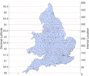
the interval we use to connect with the model (see Figure 6). In simulations, we work with
500 discrete and equally-sized ‘parishes’ that make up the whole, so the interval in the
figures are mapped into this [0,500] interval for comparison to simulation output. Also
shown in Figure 6 are the decimal latitudes that we use to refer to locations in the data
[image:23.595.115.481.336.647.2]and in simulation output.
Figure 6: England and Wales Interval
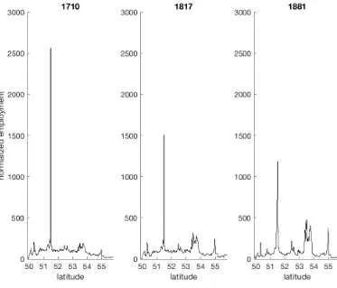
Despite this simplification of the data, many parts of the occupational geography are recognizable in the interval representation. Figure 7 depicts normalized total employment
mapped into the interval at three dates.15 Evident in the figure around latitude 51.5◦ is
the city of London. Also visible is the growth in the labour employed in the North of
England around 53.5◦ and the relative decline in dominance of London. The interval
permits an understanding of both the geographical distance from London to the hotspot
in the North and of the magnitude of the shift of employment from the South to the
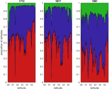
North. One way to look at the occupational structure using the interval representation is
to consider the occupational structure at each location. Figure 8 shows this at three dates. While the secondary sector remains relatively stable over the period, the primary sector
becomes increasing spatially concentrated. This is a result of the growth of the tertiary
sector that occurs most rapidly after 1817 and, strikingly, occurs all over the country.
This points to the particular role of the tertiary sector in transport and distribution of
the increased output of the primary and secondary sectors; it grows in importance both
[image:24.595.118.491.329.648.2]withinand between cities. It also shows that the features seen in the 2-dimensional maps (Figures 2–4) are replicated in the 1-dimensional interval representation.
Figure 7: Interval distribution of total employed (normalized)
Figure 8: Sector Proportions (bottom to top: primary, secondary,tertiary)
4.2
Parameterization
To parameterize the initial spatial distribution of productivity in primary and secondary
sectors, we use the 1710 spatial distribution of employment in each sector. In particular,
we invert the production functions, equations (3)-(4), to obtain an expression for local
productivity as a function of labour, prices and wages at each location. We then use observations for labour employed along with prices and wages which solve the model. Since
the initial spatial diffusion of technologies in the model creates a jump in productivity
levels (both on aggregate and spatially), we report model output starting att = 1 after a
t= 0 diffusion of technology in each sector. (see Trew, 2014, for more detail).
The baseline parameterization is given in Table 1. We select ζ and r to fit the initial
aggregate level and spatial distribution of tertiary labour in the model to that observed
in the data. Setting r <1 captures a substitutability between labour and infrastructure
stock in the production of transportation services. The preference parametersηandγ are
chosen to match the initial share of labour in agriculture and manufacturing as well as the extent of the shift out of agriculture over the period. We use Valentinyi and Herrendorf
(2008) to pin-down the production parameters α and µ; as described above, µ > α since
agricultural production is relatively more land-intensive. The Pareto parameters,aM and
there was a long, slow growth agricultural productivity in the period leading up to the
industrial revolution; aA captures a near-doubling of productivity every 150 years. The
manufacturing innovation parameter, aM, generates a long-run manufacturing growth
rate of 2% as in Crafts and Harley (1992). The fixed and marginal costs for innovation
are chosen to, first, begin at t = 1 (year 1710) with some agricultural innovation and,
second, to pin down the timing of the takeoff of manufacturing innovation in the baseline simulation. The diffusion decay parameter,δ, affects the pace of takeoff and so we choose
[image:26.595.108.494.234.604.2]is to match the evidence in Crafts and Harley (1992).
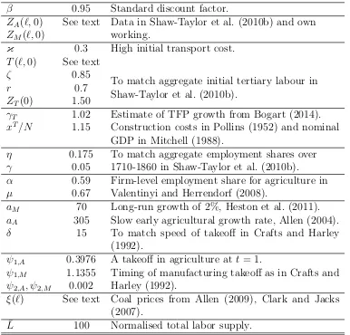
Table 1: Parameterisation for baseline model
β 0.95 Standard discount factor.
ZA(`,0) See text Data in Shaw-Taylor et al. (2010b) and own
working.
ZM(`,0)
κ 0.3 High initial transport cost.
T(`,0) See text
ζ 0.85
To match aggregate initial tertiary labour in Shaw-Taylor et al. (2010b).
r 0.7
ZT(0) 1.50
γT 1.02 Estimate of TFP growth from Bogart (2014).
xT/N 1.15 Construction costs in Pollins (1952) and nominal
GDP in Mitchell (1988).
η 0.175 To match aggregate employment shares over 1710-1860 in Shaw-Taylor et al. (2010b).
γ 0.05
α 0.59 Firm-level employment share for agriculture in Valentinyi and Herrendorf (2008).
µ 0.67
aM 70 Long-run growth of 2%, Heston et al. (2011).
aA 305 Slow early agricultural growth rate, Allen (2004).
δ 15 To match speed of takeoff in Crafts and Harley (1992).
ψ1,A 0.3976 A takeoff in agriculture att = 1.
ψ1,M 1.1355 Timing of manufacturing takeoff as in Crafts and
Harley (1992).
ψ2,A, ψ2,M 0.002
ξ(`) See text Coal prices from Allen (2009), Clark and Jacks (2007).
¯
L 100 Normalised total labor supply.
The initial transport parameter is set at κ = 0.3. This means an initial physical
transport cost of 0.11 (compared with κ = 0.008 in DR-H) to capture the large costs to
transporting goods in the early 18th century. We set T(`, t) to be fixed for all t at the
initial distribution of access to transport in 1710.16 For energy prices, we use data in Clark and Jacks (2007) and Allen (2009) on the relative price of coal at different locations
16At 1710 there is some variation in access to early turnpikes and navigable rivers. The calculation of
in 1700. In counterfactual exercises below we vary the initial distribution of the coal price
and interact it with developments in transport costs.
4.3
Simulation output
Results from using the baseline calibration are reported in Figures 9-15. In each figure,
the thick line is a mean average of 100 simulations with shading to represent a confidence
interval of two standard deviations around the mean. Since the model incorporates a
con-tinuum of firms, the randomness of innovation realizations should disappear on aggregate in a single run. However, as in DR-H, we model a finite number of discrete intervals that
each receive the same innovation realization. That the confidence intervals are relatively
tight to the mean model output suggests that the chosen number of discrete intervals
is enough to ensure that separate runs of the model do not generate widely different
outcomes.
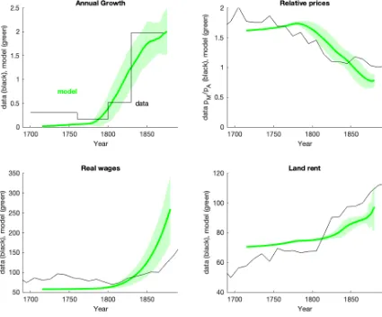
Figure 9 gives the performance of the model in terms of a number of macroeconomic
variables. The takeoff in growth matches the timing and magnitude of that reported in
Mokyr (2004). The relative price of manufactured goods captures the decline observed in
the data (calculated using the method in Yang and Zhu, 2009). The path of real wages and average land rent is consistent with the data in Clark (2002) although with perhaps
too much increase in real wages and too little increase in land rents.
In terms of the aggregate structural transformation, Figure 10 demonstrates some
success in matching the data described in Section 2. Employment in the secondary
sec-tor exhibits a slow, steady increase over the whole period. This is despite that secsec-tor
generating the increases in productivity that underpin the takeoff in growth. The more
rapid decline of the primary sector after 1800 is accompanied by a larger acceleration in
the employment of the tertiary sector. The driver of this change is the increased
out-put and trade referred to by Shaw-Taylor et al. (2010b) which in the model causes a greater demand for transportation services. Absent the endogenous tertiary sector, the
model would not explain the slow change in the relative importance of the secondary
sector alongside the fast change in the relative importance of the primary. As is clear,
the growth in the relative importance of tertiary labour outstrips that in the data and a
consequence is that the primary sector falls too much and the secondary sector grows too
little. Since infrastructure is fixed in this version of the model, landowners can respond
to the increased demand for transport services only by hiring more labour. As we will see
in Section 5, when we permit investments in fixed infrastructure, some of the pressure on
tertiary labour can be relieved by investment in infrastructure improvements.
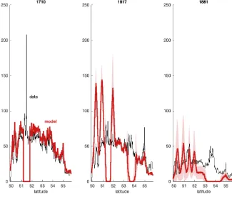
The benefit of using a model that incorporates continuous space is that it can be compared against data that offers a high spatial resolution. To that end, Figure 11 plots
Figure 9: Baseline Simulation: Macroeconomic Variables
Figure 10: Baseline Simulation: Structural Transformation (% labor share)
(Average of 100 simulations±2s.d.)
three dates (1710, 1817 and 1881).17 Productivity growth in the agricultural ‘south’ of the
interval (over the latitude range of roughly 50.5◦to 52◦) occurs endogenously as firms there
are initially larger and can amortize the fixed costs of innovation. This causes primary
output to specialize in the south in a way that mirrors the data, although less clearly in
1881, and which is consistent with the literature (Allen, 2004). The localized agricultural
innovations cause labour to be more concentrated than in the data. The eventual decline
in the southern primary workforce in response to the shift toward manufactured goods
matches that in the data. However, the complete primary-secondary specialization in
each location means that the model misses some primary employment in the South at 1710 and some primary employment in the North at 1881. Figure 8 places the data in
Figure 11 in context – while there are areas of high primary employment shares in the
North, they decline in relative terms as the secondary sector grows. For example, the high
primary employment level in 1881 around latitude 53.5◦ is only around one sixth of the
level of secondary employment at the same location. The model captures the relatively
high share of primary employment in the South and, as we see below, the relatively high
share of secondary employment in the North. Moreover, the specialization is not critical
17The discrepancy between 1710 and 1817 at around 51.5 in Figure 11 is a result of the reconstruction
for the ability of the model to capture the industrial takeoff – the model captures a
slow agricultural revolution in the South in spite of missing some primary employment in
[image:30.595.137.462.159.439.2]London at 1710.
Figure 11: Baseline Simulation: Primary Employment
(Average of 100 simulations±2s.d.)
As the agricultural revolution proceeds in the south, consumption demand, and so
labour employed, shifts towards manufacturing firms. That raises the optimal size of
manufacturing firms and makes them more likely to be able to offer land rents in excess of
those offered by agricultural firms. The growing scale of manufacturing firms also means
they may amortize the fixed cost of innovation over a larger output, while because of
the scale-effect in equation (9) the innovation intensity increases. At t = 72 (year 1782), manufacturing firms at latitude 53.7 find it optimal to invest in innovation. Thereafter, the
innovation-driven industrial revolution proceeds; aggregate growth increases and the shift
of consumption out of agriculture accelerates. As Figure 12 shows, labour in the secondary
sector moves toward a northern hotspot. The location of this industrial hotspot matches
the data, though the size of the takeoff in the model is in excess of that in the data. The
secondary employment in the model also predicts that London (around latitude 51.4◦),
declines more than in the data. In reality, of course, London continued to be an important
centre of activity throughout the eighteenth and nineteenth centuries. However, there are
a number of things not in the model that make London different. Following its founding
eventually forming a large part of the first financial revolution following the Glorious
Revolution in 1688. Its principal sources of employment throughout this period were
not those sectors that underpinned the industrial revolution. As the model is of only
one sector, a better comparison is to the single sector, textiles, that during this period
drove industrial growth. As Figure 13 shows, the model captures the location, timing
and magnitude (once rescaled) of the takeoff in textiles employment. Moreover, we can consider whether the model would still be able to capture the endogenous emergence of a
Northern hotspot if London were arbitrarily forced to persist. What triggers the rise of the
industrial hotspot in the North is a steady increase in the relative price of manufactured
goods that results from the slow agricultural revolution in the South. With an arbitrary
‘capital employment’ in the secondary sector added to the model around 51.4◦, we would
still see this change in relative prices so long as the agricultural revolution in the South
[image:31.595.141.461.336.610.2]occurs.
Figure 12: Baseline Simulation: Secondary Employment
(Average of 100 simulations±2s.d.)
Finally, we can consider the spatial fit of the model to the tertiary employment data.
As Figure 14 shows, the model does well in matching much of the local tertiary employ-ment, particularly in the initial period and in the industrial hotspot that emerges. The
model does less well in others (such as, again, in London). The model prediction for
the transport labour in the industrial region is greater than that in the data, again since
Figure 13: Baseline Simulation: Textiles Employment (rescaled)
(Average of 100 simulations±2s.d.)
of the dynamism of the tertiary sector was shown in Figures 4 and 8, that the growth
of the tertiary sector grew as a proportion of local employment in a highly uniform way.
As Figure 15 shows, the model is able to explain the uniform upward shift in the share
of tertiary employment across the interval.18 This is quite distinct from the model impli-cations for the primary and secondary sectors which mirror the data in concentrating in
one region. The model over-estimates the share in the middle of the interval. This partly results from the assumption that goods are traded wholly across the land. As a result, the
model predicts that the accumulated traded good peaks around 53.1◦. In reality, some
trade would take place in coastal shipping which would connect points in the South with
the North without inducing transport labour demand in the Midlands. In being able to
match the data with the tertiary sector explained as a function of output and trade in the
other sectors, the findings are consistent with the hypothesis presented in Shaw-Taylor
et al. (2010b).
18Appendix Figures 21-22 report similar figures with shares for the primary and secondary sectors.
Figure 14: Baseline Simulation: Tertiary Employment
(Average of 100 simulations±2s.d.)
Figure 15: Baseline Simulation: Tertiary Shares
[image:33.595.144.456.470.730.2]