Munich Personal RePEc Archive
Business cycle determinants of US
foreign direct investments
Cavallari, Lilia and D’Addona, Stefano
December 2012
Online at
https://mpra.ub.uni-muenchen.de/43616/
Business cycle determinants of US foreign direct
investments
Lilia Cavallari
∗Stefano D’Addona
†Abstract
This paper investigates the role of output fluctuations and exchange rate volatil-ity in driving US foreign direct investments (FDI). Using a sample of 46 economies over the period 1982-2009, we provide evidence of a positive relation between US FDI and host country’s cyclical conditions. Allowing for asymmetry over the busi-ness cycle, we find that the output elasticity of foreign investments is higher in booms than in recessions. An increase in exchange rate volatility, on the other hand, has a strong deterrent effect on US foreign investments. This effect is fairly stable over the business cycle.
JEL classification: F21, E22, F42.
Keywords: FDI, business cycle, cyclical output, exchange rate volatility.
1
Introduction
This paper investigates the impact of the business cycle on US foreign direct investments (FDI) in a sample of 46 countries over the period 1982-2009. Most empirical studies on the determinants of FDI overlook cyclical factors.1
Yet, there are good reasons why the business cycle might influence foreign investments. On the theoretical ground, two main channels have been identified. In models with capital market imperfections `a la Bernanke et al., 2000, a mechanism of financial accelerator typically leads to pro-cyclical invest-ments, i.e. a positive correlation between investment and output. The reason is a rise in the cost of borrowing which depresses investments in cyclical downturns (for extensions to an international setting, see Gilchrist et al. 2002 and Faia, 2010). Early attempts to investigate the role of a firm’s borrowing opportunity for financing an investment overseas have mainly focused on the link between exchange rates and FDI (Froot and Stein, 1991). Unfortunately, the relation between aggregate FDI flows and exchange rates appears to be far from conclusive. 2
In a setup with firm entry, business cycle conditions may affect entry costs as well as investment revenues with potential contrasting effects on the decision whether to access foreign markets in the first place. 3
Consider for instance a productivity drop in the country of destination of foreign investments. This deteriorates the prospective revenues from overseas investments, thereby discouraging entry of new firms. The fall in produc-tivity, however, may well reduce the entry costs faced by multinational firms, for instance because of a strong depreciation of the foreign currency. The effect on entry is clearly reversed. In a similar vein, Russ, 2007 shows that an increase in interest rate volatility may in principle attract or deter foreign investments depending on whether it originates in the host or in the source country. Empirical research has recently addressed the question, finding encouraging results in favour of a role of macroeconomic uncertainty in shaping entry decisions by multinational firms.4
Regarding overall FDI activities, the evidence so far suggests that they do respond to macroeconomic fluctuations over the cycle.5
Our knowledge, however, is still limited as concerns the contribution of different sources of business cycle volatility and the channels through which they affect foreign investments. In a companion paper, Cavallari and D’Addona, 2013 make a first step towards clarifying the role of nominal and real volatility. In a sample of OECD economies, we find that an increase in volatility has a negative effect on foreign investments independently of the underlying source of uncertainty. Output and
1
They typically focus on factors that are relatively persistent over time. These include various measures of business attractiveness, ranging from market size to cultural ties and institutional variables, as well as proxies of the cost of foreign market access. Comprehensive surveys of the literature include Razin and Sadka, 2004, Blonigen 2005 and Bloniger and Piger, 2010, among others.
2
Stevens, 1998 shows that the relation between FDI and exchange rates is highly unstable. Cush-man (1985, 1988), Goldberg and Koldstadt, 1995 and Zhang, 2003 find a positive effect of exchange rate volatility on FDI. Evidence of a negative effect is provided, among others, by Campa, 1993 and Chakrabarti and Scholnick, 2002.
3
See, among others, Helpman et al. 2004, Russ, 2007, Cavallari (2007, 2010) and Lewis, 2010.
4
See Russ, 2012 and Russ and Lubik, 2012.
5
exchange rate volatility matter in particular for the decision whether to invest in a foreign country in the first place. Interest rate volatility, instead, mainly influences the amount of overseas investments.
In this paper, we adapt the empirical strategy in Cavallari and D’Addona, 2013 to a context of unilateral FDI flows. We investigate the effect of the business cycle in the country of destination of US foreign investments, focusing on cyclical output and nominal volatility. The former captures medium-frequency output fluctuations using a Hodrick Prescott filter, as is standard practice in business cycle studies. The latter is meant to represent uncertainty over monetary policy. We consider the coefficient of variation of nominal exchange rates towards the US dollar. The rest of the paper is organized as follows. Section 2 describes our empirical strategy and discusses the results. Section 3 contains the conclusions.
2
Empirical analysis
2.1
The baseline regression
Our baseline regression is:
log(F DIh,t) = α+βcycleh,t +γvolh,tN +δZt+uh,t (1)
where F DIh,t is the outflow of FDI from the US to country h (host) at time t,cycleh,t is
cyclical output in the host country, volN
h,t an indicator of nominal volatility, Zt a matrix
of control variables to be specified below and uh,t is an error term. We estimate equation
(1) using a panel estimator with random effects, corrected for heteroskedasticity in the residuals. 6
As is standard practice in gravity models, we use the log of the dependent variable. This reduces the weight of outliers and simplifies the interpretation of coefficients as elasticities. Taking the log is, however, problematic with FDI data (in our sample, 202 out of 1187 observations are negative). Following Levy Yeyati et al. (2007), we therefore use the semi-log transformation:
[
F DI =sign(F DI) log(1+|F DI |)
The transformation above has the advantage of preserving the sign of FDI flows at the cost of time-varying elasticity estimates. For large values of the dependent variable, however, this cost is small (equivalent to 1 dollar per unit of FDI flow in our data) and the coefficients can be safely interpreted as (semi) elasticities.
The indicator of nominal volatility (volN) is meant to capture uncertainty in monetary
policy. For ease of comparison with earlier studies stressing the role of exchange rates, we consider exchange rate volatility as measured by the coefficient of variation of monthly nominal exchange rates in domestic currency vis `a vis the US dollar. In our specification, an increase in nominal volatility includes both the within-country (i.e., the change over
6
The Hausman test rejects the null that the fixed and random effect models are equivalent with a p-value of 0.93. The Breusch Pagan test does not reject the null of random effects against the alternative OLS model. Post estimation tests reject the hypothesis of autocorrelation in the residuals (Wooldridge test) while not rejecting that of heteroskedasticity (log-likelihood ratio test).
time) and the between-country effect (i.e., the change across countries). Since both effects reduce the expected profitability of foreign investments, we expect a negative sign for γ. Cyclical output is identified with a HP filter, (Hodrey and Prescott, 1997), as is common in business cycle studies. A boosting cycle (i.e., a positive value of the variable
cycle) has a positive effect on foreign investments both within-country (positive income effect) and between-country (positive substitution effect). Therefore we expect a positive
β.
Finally, we control for time invariant variables, as distance, common language and border, as well as for country’s size (the log of population) in the spirit of the gravity model (Anderson, 1979). To account for differences in monetary conditions across countries, we also include inflation in matrix Z.
2.2
Data
FDI data are from the Bureau of Economic Analysis Direct Investment & Multinational Companies (MNCs) Database7
. They comprise annual FDI flows from US to 46 economies from 1982 to 2009.8
FDI flows represent the total equity outflow from each country to any other country in the sample, including retained earnings and intra-firm transfers. Negative flows represent disinvestments. FDI in current dollars are deflated using the US GDP deflator.
Data on exchange rates and real and nominal GDP are from the OECD’s Main Eco-nomic Indicators (MEI) Database. Exchange rate volatility is the coefficient of variation of monthly nominal exchange rates in foreign national currency vis `a vis the US dollar. As is standard practice in business cycle studies, cyclical fluctuations are identified by a filter that decomposes original data by frequency band. Our measure of cyclical output is the Hodrick and Prescott, 1997 filter.
Finally, the control variables comprise: distance, population, inflation, the log of real GDP and two dummies for common language and common border.9
2.3
Results
[Table 1 about here.]
As a preliminary analysis, we estimate the baseline regression in equation (1) with-out controls. The estimates, reported in table 1 are calculated with fixed (cf. column 1) and random effects (cf. column 2), correcting the errors for autocorrelation and het-eroschedasticity. While the coefficients are almost identical in the two specifications, the Hausman test rejects the fixed effect model. In the remainder, we therefore focus on the random effect specification. Looking at the business cycle indicators, the preliminary re-sults provide interesting insights on the cyclical behavior of US FDI. Both the coefficients of interest are significant and with the expected sign.
7
http://www.bea.gov.
8
The list of the countries includes all the OECD current members (cf. http://www.oecd.org) excluding Chile, Estonia, Slovak Republic, and Slovenia. No OECD members included in the dataset are Argentina, Brazil, China, Hong Kong, India, Indonesia, Jamaica, Kuwait, Panama, Peru, Philippines, Romania, Russia, Saudi Arabia, Singapore, Thailand and Venezuela.
9
The coefficient on cyclical output suggests that a 1% increase of output over the trend raises average US investments abroad by roughly .08%. Such a moderate effect does not come as a surprise if we consider that the coefficient β captures the net effect of output fluctuations above and below the trend. As long as output fluctuations have asymmetric effects over the cycle (for instance, stronger in booms than in recessions) the coefficient might turn very small. We will investigate the extent of asymmetry later on. An increase in exchange rate volatility, on the contrary, has a strong deterrent effect. A 1 percent rise in nominal volatility (calculated both within and across countries) reduces US investments abroad by 1.35% on average.
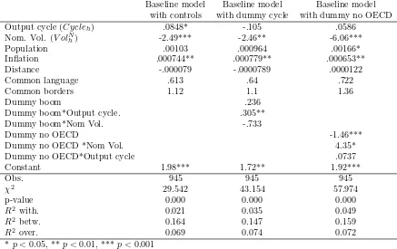
Results are confirmed when we add a set of controls to account for market size and inflation in the host country as well as for physical and cultural proximity with the US. Estimates, reported in the first column of table 2, show that the coefficient on cyclical output remains unchanged while the effect of nominal volatility is stronger (predicting a drop of 2.49% for a 1% increase in exchange rate volatility).
As said above, a low elasticity might reflect asymmetries in the response of investment decisions over the cycle. To assess the issue in more detail, our baseline model is aug-mented with an indicator variable that takes on a value of 1 when the difference between cycle and trend is positive (i.e., in a “boom”) and a value of 0 otherwise. We interact the dummy boom with both nominal volatility and cyclical output. A significant coefficient of the dummy means a change in the average level of FDIs over the cycle. A positive coefficient, for instance, means that average investments are higher in booms than in re-cessions. By the same token, a significant coefficient on the interaction terms reflects a change in the elasticity of FDI with respect to the interacted variable.
Results, reported in the second column of table 2, suggests that asymmetry indeed plays a role. The response of US FDI to a 1% increase in the host country’s output is positive and significant only when the latter is interacted with the dummy variable, namely when there is a boom in the destination country. Moreover, it is almost 4 times as large as in the baseline model. The intuition is that “bad news are no news”: US foreign investments increase when the host country is in a boom (with elasticity equal to 0.3) while not reacting at all in recessions. This behavior might reflect high costs of disinvestment. Booming conditions in the host country, on the other hand, do not influence neither the average amount of US foreign investments nor their elasticity to exchange rate volatility.
[Table 2 about here.]
Finally, we investigate whether there are differences in US FDI towards OECD and non-OECD members. For that purpose, we construct the dummy “no OECD” which takes on a value of 1 when the host country is a non-OECD member and a value of 0 otherwise. As before, the dummy variable is interacted with both nominal volatility and cyclical output, providing a comparable interpretation in terms of average and elasticity effects. Table 2, third column reports the results. On average, US FDI outflows to non-OECD members are significantly less than those to non-OECD members.10
The finding is in line with a general tendency towards an intensification of investments among “similar” economies in the last decades (UNCTAD 2011). Interestingly, the elasticity to nominal volatility is higher among OECD countries (equal to -6.06) than that among non-OECD members (equal to -1.71). The finding might reflect a much higher exchange rate volatility in non-OECD countries compared to that in OECD economies.
10
The drop in the average amount of FDI is as large as 1−e1
.92−1.46
e1
.92 ≈77%.
3
Conclusions
Using a sample of 46 countries over the period 1982-2009, this paper investigated the role of business cycle fluctuations and exchange rate volatility in driving US FDI flows.
In particular, we provide evidence of a positive relation between cyclical output in the host country and US foreign investments. This relation appears to be stronger in booms than in recessions, supporting the view that “bad news are no news” as far as disinvestments are concerned.
As regards nominal volatility, we find that an increase in exchange rate volatility strongly deters US foreign investments. The coefficient on nominal volatility is fairly stable over the business cycle while being higher among OECD countries compared to non-OECD economies.
References
[1] Anderson, J.E. 1979. A theoretical foundation for the gravity equation. American Economic Review 1979, 69 (1), 106-116.
[2] Bernanke, B.S., M. Gertler, and S. Gilchrist 2000. The financial accelerator in a quan-titative business cycle framework. In: Taylor, J., and M. Woodford (eds.), Handbook of Macroeconomics, Amsterdam, North Holland, chapter 21.
[3] Blonigen B., 2005. A review of the empirical literature on FDI determinants.Atlantic Economic Journal 33, 383-403
[4] Blonigen B. and J. Piger, 2010. Determinants of FDI.NBER working paper no. 16704
[5] Buch C. and Lipponer, 2005. Business cycle and FDI: evidence from German sectoral data.Review of World Economics(Weltwirtshaftlihes Archiv) 2005, 141 (4), 732-759.
[6] Campa J., 1993. Entry by foreign firms in the United States under exchange rate uncertainty. The Review of Economics and Statistics 1993, 75 (4), 614-622.
[7] Campa J. and L. Goldberg, 1995. Investments in manufacturing, exchange rates and external exposure, Journal of International Economics 1995, 38, 1995, 297-320.
[8] Cavallari L., 2007. A macroeconomic model of entry with exporters and multination-als. The B.E. Journal of Macroeconomics 2007, 7(1), Contributions, Article 32.
[9] Cavallari L., 2010. Exports and FDI in an endogenous-entry model with nominal and real uncertainty. Journal of Macroeconomics 2010, 32, 300-313.
[10] Cavallari L. and S. D’Addona, 2013. Nominal and real volatility as determinants of FDI. Applied Economics, 45:18, 2603-2610
[12] Cushman, D., 1985. Real exchange rate risk, expectations and the level of direct investment. The Review of Economics and Statistics 1985, Vol. 67, No. 2, pp. 297-308.
[13] Cushman D., 1988. Exchange rate uncertainty and foreign direct investments in the United States. Review of World Economics (Weltwirtshaftlihes Archiv) 1988, 124, 322-335.
[14] Faia, E. 2010. Financial frictions and the choice of exchange rate regimes. Economic Inquiry 2010, Vol.48, No. 4, pp. 965-982.
[15] Froot, K.A. and J.C. Stein 1991. Exchange rates and foreign direct investment: an im-perfect capital markets approach.The Quarterly Journal of Economics 1991, 106(4), 1191-1217.
[16] Gilchrist, S., J.O. Hairault, and H. Kempf 2002. Monetary policy and the financial accelerator in a monetary union. European Central Bank Working Paper 175.
[17] Goldberg, Linda S. and Charles D. Kolstad 1995. Foreign direct investment, exchange rate variability and demand uncertainty, International Economic Review 1995, Vol. 36, No. 4, pp. 855-873.
[18] Helpman E., Melitz M. and S. Yeaple, 2004. Export versus FDI with heterogeneous firms. American Economic Review 2004, 94(1), 300-316.
[19] Hodrick, Robert and Edward Prescott, 1997. Post-war US business cycles: An em-pirical investigation. Journal of Money, Credit, and Banking 1997, 29, 1ˆae“16.
[20] Holzl, Werner, 2005. Tangible and intangible sunk costs and the entry and exit of firms in a small open economy: the case of Austria.Applied Economics 2004, 37(21) , 2429-2443.
[21] Levy Yeyati, E., U. Panizza, and E. Stein 2007. The cyclical nature of north-south FDI flows. Review of International Economics 2007, 15(1), 146-163.
[22] Lewis L.T., 2010. Exports versus multinational production under nominal uncer-tainty. Mimeo, University of Michigan.
[23] Razin A. and E. Sadka, 2007, Foreign direct investment: analysis of aggregate flows. Princeton University press. Princeton, 08540, NJ.
[24] Russ K., 2007. The endogeneity of the exchange rate as a determinant of FDI: a model of money, entry and multinational firms. Journal of International Economics
2007, 71, 344-372.
[25] Russ K., 2012. Exchange rate volatility and first-time entry by multinational firms.
Review of World Economics, 148, 2, 269-295.
[26] Russ K. and T. Lubik, 2012. Exchange rate volatility in a simple model of firm entry and FDI. Economic Quarterly, Federal Reserve Bank of Richmond, issue 1Q, 51-76.
[27] Stevens G., 1998. Exchange rates and foreign direct investments: a note. Journal of Policy Modeling 1998, 20 (3), 393-401.
[28] UNCTAD, 2007. World investment report.
[29] Wang M. and S. Wong, 2007. Foreign direct investment outflows and business-cycle fluctuations. Review of International Economics 2007, 15(1), 146-163.
Table 1: Baseline regression with no controls
This table reports the estimates of the baseline model in equation (1) without any control variable. The dependent variable is the semi-log trasformation of FDI outflows expressed in real dollars.
Fixed effects Random effects Output cycle (Cycleh) .0822** .0823**
Nom. Vol. (V olN
h) -1.34** -1.35**
Constant 1.69*** 1.64***
Obs. 1173 1173
F stat. 8.627
χ2
17.604
p-value 0.000 0.000
Hausman test χ2
(2) = 0.04, Prob> χ2
= 0.981
R2
with. 0.015 0.015
R2
betw. 0.008 0.008
R2
over. 0.013 0.013
* p <0.05, **p <0.01, *** p <0.001
Table 2: Baseline regression with controls and dummies for the business cycle and OECD membership
This table reports the estimates of the baseline model in equation 1 augmented with control variables (first column). The second column reports the same estimates adding a “dummy” variable to capture the phases of the business cycle, while the third column reports the estimates adding a “dummy” variable to capture OECD membership. The dependent variable is the semi-log transformation of FDI outflows expressed in real dollars.
Baseline model Baseline model Baseline model with controls with dummy cycle with dummy no OECD Output cycle (Cycleh) .0848* -.105 .0586
Nom. Vol. (V olN
h) -2.49*** -2.46** -6.06***
Population .00103 .000964 .00166*
Inflation .000744** .000779** .000653**
Distance -.000079 -.0000789 .0000122
Common language .613 .64 .722
Common borders 1.12 1.1 1.36
Dummy boom .236
Dummy boom*Output cycle. .305**
Dummy boom*Nom Vol. -.733
Dummy no OECD -1.46***
Dummy no OECD *Nom Vol. 4.35*
Dummy no OECD*Output cycle .0737
Constant 1.98*** 1.72** 1.92***
Obs. 945 945 945
χ2
29.542 43.154 57.974
p-value 0.000 0.000 0.000
R2
with. 0.021 0.035 0.049
R2
betw. 0.164 0.147 0.159
R2
over. 0.069 0.074 0.072