Munich Personal RePEc Archive
Causal linkages between electricity
consumption and GDP in Thailand:
evidence from the bounds test
Jiranyakul, Komain
National Institute of Development Administration
November 2014
Online at
https://mpra.ub.uni-muenchen.de/60625/
Causal Linkages between Electricity Consumption and GDP in
Thailand: Evidence from the Bounds Test
Komain Jiranyakul, School of Development Economics, National Institute of Development Administration, Thailand. Email: komain_j@hotmail.com
Abstract: This paper investigates the causal relationship between electricity consumption and real GDP by applying the bounds testing for cointegration in a multivariate framework. The error correction mechanism is employed to detect causal relationship in the presence of cointegration among three variables. Empirical results for Thailand during 2001Q1 and 2014Q2 suggest that there is long-run unidirectional causality between electricity consumption and real GDP. The source of causation in the long run is found by the significance of the error correction terms in the Wald F-test. In the short run, bidirectional causal relationship between electricity consumption and economic growth is observed. The findings give implications for electricity efficiency and alternative energy sources in the long run.
Keywords: Causality, electricity consumption, economic growth
JEL Clasification: Q43, C32
1. Introduction
Previous studies investigate the impact of energy consumption on real GDP using popular cointegration techniques to find a long-run relationship between the two variables. Both short-run and long-run causality have been examined in advanced and developing or emerging market economies. There can be unidirectional or bidirectional causality between energy and GDP. It is also possible that the neutrality hypothesis exists, i.e., energy consumption does not cause GDP or GDP does not cause energy consumption. Earlier study by Kraft and Kraft (1978) shows that energy consumption Granger causes GNP in the United States during 1947 and 1974. However, Yu and Jin (1992) and, among others, find a long-run causality of energy consumption to output while Glausure and Lee (1997) find bidirectional causality between energy consumption and GDP in South Korea and Singapore. Asafu-Adjaye (2000) estimates the causal relationships between energy consumption and income for India, Indonesia, the Philippines and Thailand. He finds unidirectional causality running from energy consumption to income in India and Indonesia and bidirectional causality in the Philippines and Thailand. Oh and Lee (2004) re-examine the causal relationship between energy consumption and real GDP in Korea over the period 1970-1999 by estimating a vector error correction mechanism to perform the Granger causality test and find a long-run bidirectional causality between energy consumption and GDP.
finds bidirectional causality between the two variables. Ho and Siu (2007) find unidirectional causality running from electricity consumption to real GDP in Hong Kong. Chen et al. (2007) find that the directions of causality between electricity consumption and real GDP are mixed among ten Asian economies when the data for individual countries are analyzed. However, bidirectional causality is found in the panel data analysis. Narayan and Smyth (2009) use a panel dataset in the Middle Eastern countries to examine the relationship between electricity consumption and GDP and find bidirectional causation between the two variables. Chandran et al. (2010) examine the relationship between electricity consumption and real GDP for Malaysia during 1971 and 2003. They find that electricity consumption, real GDP and price are cointegrated. In addition, there is a unidirectional causality running from electricity consumption to economic growth. Sami (2011) finds that real per capita income causes electricity consumption in Japan. Faisal and Nirmalya (2013) find that electricity consumption does not cause growth in India, but there is bidirectional causality between the two variables in Pakistan. Halkos and Tzeremes (2014) use a sample of 35 countries over the 1990-2011 period to examine the relationship between electricity consumption from renewable sources and GDP. They find that electricity consumption from renewable sources will not cause higher GDP in emerging and developing countries.
The main objective of the present study is to examine the causal links between electricity consumption and real GDP in Thailand. The available data from 2000Q1 to 2014Q2 are used. The bounds test or autoregressive distributed lag (ARDL) procedure is employed. The main finding is that there is long-run bidirectional causality between real GDP and electricity consumption. The paper is organized as the following. The next section presents the data description and method of estimation. Section 3 gives empirical results. The final section concludes.
2. Data and Methodology
Quarterly data during 2000Q1 and 2014Q2 are used in the analysis. The data of electricity consumption are obtained from Electricity Generating Authority of Thailand and Provincial Electricity Authority, Ministry of Interior. Energy price index series is obtained from Bureau of trade and economic indices, Ministry of commerce. Real GDP series is obtained from the office of National Economic and Social Development Board. These available data are also tabulated by the Bank of Thailand. Energy consumption is measured in billion kilowatt hours while GDP at 1988 constant prices is measured in billions of baht. All series are transformed to logarithmic series. The number of observations is 58.
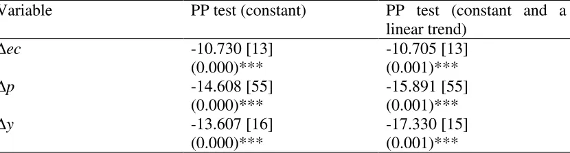
The stationarity property of the data is tested using the PP tests by Phillips and Perron (1998) on first differences of the series and the results are shown in Table 1.
Table 1 Results of unit root tests
Variable PP test (constant) PP test (constant and a linear trend)
∆ec -10.730 [13] (0.000)***
-10.705 [13] (0.001)***
∆p -14.608 [55]
(0.000)***
-15.891 [55] (0.001)***
∆y -13.607 [16]
(0.000)***
-17.330 [15] (0.001)***
Note: ∆ denotes first difference operator. The variables: ec is electricity consumption, p is energy price index, and y is real GDP. The number is bracket is optimal bandwidth determined by Bartlett kernel. The number in parenthesis is the probability of accepting the null hypothesis of unit root. *** indicates significance at the 1 percent level.
The results in Table 1 ensure that the maximum order of integration of the three variables is one because the null hypothesis of unit root is rejected. Therefore, the bounds test is applicable to the data. This bounds test can provide unbiased long-run estimates and valid test statistics. The long-run equilibrium relationship between energy consumption, consumer price index and manufacturing production can be express as:
ect =α10 +α11pt +α12yt +e1t (1)
pt =α20 +α21ect +α22yt +e2t (2)
yt =α30 +α31ect +α32pt +e3t (3)
where ∆ denotes first difference operator, ec is the log of electricity consumption, p is the log of energy price index, and y is the log of real GDP. Equation (1) represents the demand side approach or electricity demand function. Because of the unavailability of electricity price series, the energy price index, denoted by p, is used as a proxy of electricity price. Chandran et al. (2010) and Oh and Lee (2004) use consumer price index as a proxy of electricity price due to the lack of the data of electricity price. Equation (2) is used to examine the impact of electricity consumption and real GDP on price while equation (3) is used to examine the impact of electricity consumption and price on real GDP.
The unrestricted error correction models of this ARDL procedure can be expressed as:
t k t p
k k p
j
j t j i
t p
i i t
t t
t a a ec a p a y ec p y
ec 1
3
0 1 2
0 1 1
1 1 1
13 1 12 1 11
10 + + + + β ∆ + γ ∆ + ϕ ∆ +ε
=
∆ −
= =
− −
= − −
−
∑
∑
∑
t k t q k k q j j t j i t q i i t t t
t a a p a ec a y p ec y
p 2 3 0 2 2 0 2 1 1 2 1 23 1 22 1 21
20 + + + + β ∆ + γ + ϕ ∆ +ε
= ∆ − = = − − = − − −
∑
∑
∑
(5) t k t r k k r j j t j i t r i i t t tt a a y a ec a p ly ec p
y 3 3 0 3 2 0 3 1 1 3 1 33 1 32 1 31
30 + + + + β ∆ + γ ∆ + ϕ ∆ +ε
= ∆ − = = − − = − − −
∑
∑
∑
(6) There are two steps in the bounds testing for cointegration. The first step is to estimate equations (4) – (6) using ordinary least squares method to determine the existence of a long-run relationship between the three variables. This is done by conducting an F test for the joint significance of the coefficients of lagged level variables. The null hypothesis H0 :ai1 =ai2 =ai3 =0,i=1,2,3 is tested against the alternative hypothesis3 , 2 , 1 , 0 :a1 ≠a2 ≠a3 ≠ i =
Ha i i i . In other words, the models in equations (4) – (6) are tested against the models without lagged level variables, which are the ARDL models, to obtain the computed F-statistics. If cointegration exists, the computed F-statistic will be larger than the upper bound critical value. If cointegration does not exist, the computed F-statistic will be smaller than the lower bound critical value. The computed F-statistic that takes the value between the upper bound and lower bound critical values will lead to an inconclusive result. The existence of cointegration gives the error correction mechanism (ECM) expressed as:
t k t
p k k p j j t j i t p i i t
t a e ec p y u
ec 1 3 0 1 2 0 1 1 1 1 1 1 1
10 + + ∆ + ∆ + ∆ +
= ∆ − = = − − =
−
∑
β∑
γ∑
ϕλ (7)
t k t
q k k q j j t j i t q i i t
t a e p ec y u
p 2 3 0 2 2 0 2 1 1 2 1 2 2
20 + + ∆ + ∆ + ∆ +
= ∆ − = = − − =
−
∑
β∑
γ∑
ϕλ (8)
t k t
r k k r j j t j i t r i i t
t a e y ec p u
y 3 3 0 3 2 0 3 1 1 3 1 3 3
30 + + ∆ + ∆ + ∆ +
= ∆ − = = − − =
−
∑
β∑
γ∑
ϕλ (9)
where eit-1 is the error correction term (ETC), which is the one-period lag of residuals
obtained from the ordinary least squares estimate of level relationship between the three variables in equations (1)-(3). The coefficient λi is the speed of adjustment
toward the long-run equilibrium. The models in equations (7) – (9) depict short-run dynamics and show how fast any deviation from the long-run equilibrium will be corrected. The significance of the coefficient of the ETC also indicates a long-run causality running from the regressors to the dependent variable. The main advantage of the conditional ARDL procedure in testing for cointegration is that re-parameterization of the model into the equivalent vector error correction model is not required compared with other techniques of cointeration tests. The ECM representations show short-run relationship between changes in levels of the three variables and their lags.
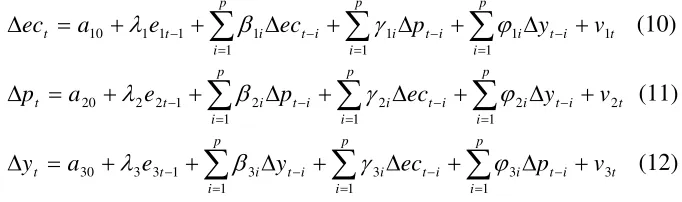
three variables. Therefore, the vector autoregressive (VAR) model augmented with the ECT can be used in stead (see Granger, 1988). The VAR model can be specified as:
t i t
p i i p i i t i i t p i i t
t a e ec p y v
ec 1 1 1 1 1 1 1 1 1 1
10 + + ∆ + ∆ + ∆ +
= ∆ − = = − − =
−
∑
β∑
γ∑
ϕλ (10)
t i t
p i i p i i t i i t p i i t
t a e p ec y v
p 2 1 2 1 2 1 2 1 2 2
20 + + ∆ + ∆ + ∆ +
= ∆ − = = − − =
−
∑
β∑
γ∑
ϕλ (11)
t i t
p i i p i i t i i t p i i t
t a e y ec p v
y 3 1 3 1 3 1 3 1 3 3
30 + + ∆ + ∆ + ∆ +
= ∆ − = = − − =
−
∑
β∑
γ∑
ϕλ (12)
If cointegration does not exist, the ECTs will be excluded from the augmented VAR model. The short-run causation can be tested by the null hopotheses Ho: γ1i=0, φ1i=0 in equation (10), Ho: γ2i=0, φ2i=0 in equation (11), and γ3i=0, φ3i=0 in equation (12). For long-run causality, the null hypotheses are the coefficients of the ECTs are zero. These Wald tests are performed by Ho and Lee (2004), and Narayan and Smyth (2009), among others.
3. Empirical Results
Since the variables may be I(0) or I(1) series, or are mutually cointegrated, the bounds test is performed to the models specified in the previous section. According to Pesaran and Shin (1999), one can obtain the preferred ECM representation in cointgeration analysis. In case of small sample size in the present study, the preferred ECMs are obtained by choosing suitable parsimonious ARDL models, which include the dummy variable, D0709t, to detect the impact of the subprime crisis on level relationships of
[image:6.595.145.486.132.233.2]the three variables. This dummy variable is defined as D0709 is 1 over the period 2007Q4-2009Q2, and zero elsewhere. The results of cointegration test are reported in Table 2.
Table 2 Results of cointegration test
Order of variable ARDL model Serial correlation (χ2(2))
Computed F
(ec, p, y) (2,1,1) 1.308
(p-value = 0.520)
6.79
(p, ec, y) (2,1,1) 2.481
(p-value = 0.289)
3.20
(y, ec, p) (2,1,0) 2.903
(p-value = 0.234)
31.66
Critical F 1 percent 5 percent 10 percent
Upper bound 7.84 4.85 4.14
Lower bound 6.48 3.79 3.17
The results from Table 2 show that the chosen ARDL models are free of serial correlation because the Chi-square statistics show that the null hypothesis of no serial correlation is accepted. When electricity consumption is the dependent variable as specified in equation (4), the computed F statistic is 6.79, which is greater than the 5% upper bound critical value of 4.85, and thus cointegration exists. On the contrary, if energy price is the dependent variable, the computed F statistic is 3.20, which is between the upper and lower bound critical values at the 10% level of significance, and the result is inconclusive. For the model with real GDP as the dependent variable, the computed F-statistic is 31.66, which is greater than the 1% upper bound critical value, and thus cointegration exists. It can be concluded that there are two cointegrating equations that should be further analyzed. Table 3 reports the results of level relationship and short-run dynamics when electricity consumption is the dependent variable.
Table 3 Results of long-run and short-run dynamics estimates of the impact of price and real GDP on electricity consumption, 2000Q1 to 2014Q2
Panel A. Long-run estimation with ect as dependent variable
Coefficient
pt 0.367 (4.730)***
yt 0.542 (4.252)***
Constant -1.865 (3.389)***
Adjusted R2 0.910
Panel B. ECM estimation with ∆ect as
dependent variable
ECT -0.349 (-2.233)**
∆ect-1 -0.112 (-0.744)
∆ect-2 -0.596 (-4.469)***
∆pt 0.116 (1.758)*
∆pt-1 0.078 (1.019)
∆yt 0.022 (0.156)
∆yt-1 -0.324 (-2.991)***
D0709t -0.039 (-2.666)**
constant 0.025 (4.168)***
Adjusted R2 0.653
Diagnostic tests:
Functional form (FF) 0.146 (p=0.702) Serieal correlation (LM) 4.043 (p=0.133) Normality (Jarque Bera) 0.024 (p=0.433) Heteroskedasticity (ARCH) 0.024 (p=0.054)
Note: The variables: ec is electricity consumption, p is energy price index, and y is real GDP. The number in parenthesis is t-statistic. p is the probability of accepting the null hypotheses that there is no serial correlation, no heteroskedasticity, and residuals are normally distributed. *** ** and * denote significance at the 1, 5 and 10 percent level, respectively.
equation illustrates the contribution of real GDP electricity consumption. The impact of price on electricity consumption is significantly positive, which implies that the economy depends on electricity regardless of the increasing trend of energy price. The short-run dynamics result from ECM estimate is illustrated in Panel B of Table 3. In the short run, the relationship between output growth and a change in electricity consumption is positive, but is not statistically significant. Furthermore, only the coefficient of lagged economic growth is statistically significant. Therefore, a change in real GDP does affect the electricity consumption in the short run. The negative impact of the subprime crisis in the short-run is visible. The estimated coefficient of the ECT is significantly negative and takes the absolute value of less than one. This indicates that any deviation from long-run equilibrium will be corrected.
The other cointegrating equation and short-run dynamics estimates are shown in Table 4.
Table 4 Results of long-run and short-run dynamics estimates of the impact of electricity consumption and price on real GDP, 2000Q1 to 2014Q2
Panel A. Long-run estimation with yt as dependent variable
Coefficient
ect 0.457 (4.252)***
pt 0.296 (3.704)***
Constant 4.011 (31.537)***
Adjusted R2 0.903
Panel B. ECM estimation with ∆yt as dependent variable
ECT -0.827 (-6.333)***
∆yt-1 0.055 (0.488)
∆yt-2 -0.235 (-2.147)**
∆ect 0.052 (0.598)
∆ect-1 -0.565 (-6.816)***
∆pt 0.094 (1.812)*
D0709t -0.012 (-1.062)
constant 0.017 (3.727)***
Adjusted R2 0.709
Diagnostic tests:
Functional form (FF) 3.083 (p=0.079) Serieal correlation (LM) 3.334 (p=0.189) Normality (Jarque Bera) 3.775 (p=0.151) Heteroskedasticity (ARCH) 0.120 (p=0.729)
Note: The variables: ec is electricity consumption, p is energy price index, and y is real GDP. The number in parenthesis is t-statistic. p is the probability of accepting the null hypotheses that there is no serial correlation, no heteroskedasticity, and residuals are normally distributed. ***, ** and * denote significance at the 1, 5 and 10 percent level, respectively.
price on real GDP is also positive. The short-run dynamics result from ECM estimate is illustrated in Panel B of Table 4. In the short run, the relationship between output growth and a change in electricity consumption is positive, but is not statistically significant. Furthermore, the estimated coefficient of lagged change in electricity consumption is positive and significant. Therefore, a change in electricity consumption does affect the growth rate in the short run. There is no impact of the subprime crisis in the short run. The estimated coefficient of the ECT (et-1) is
significantly negative and takes the absolute value of less than one. This indicates that any deviation from long-run equilibrium will be rapidly corrected.
It should be noted that the preferred ECMs are chosen because they pass the four main diagnostic tests. The Granger causality test results are reported in Table 5.
Table 5 Results of Granger causality tests Dependent
variable
Short-run causality Long-run
causality
∆ec ∆p ∆y ECT
∆ec - 7.497***[+]
(0.002)
20.624***[+] (0.000)
7.422*** (0.009)
∆p 0.358 [+] (0.701)
- 1.764 [+] (0.182)
-
∆y 17.967***[+] (0.000)
4.300**[+] (0.014)
- 0.210
(0.650)
Note: The Wald F-statistic is reported with the probability of accepting the hull hypothesis. [+] indicates a positive causation. *** and ** denote significance at the 1 and 5 percent level.
Using the Wald test, the results show that there is long-run unidirectional causality running from real GDP to electricity consumption because the coefficient of the ECT is significant at the 1 percent level. On the contrary, the coefficient of the ECT is not significant when ∆y is a dependent variable. Therefore, there is no long-run causation running from electricity consumption to real GDP. However, there is positive short-run bidirectional causality between electricity consumption and real GDP in Thailand. The findings are consistent with the results found by Sami (2011), but contradictory to Ho and Siu (2007). The results also disprove the electricity neutrality hypothesis.
The findings in the present study give policy implications for the country, including some other emerging market economies. Since the economy is dependent on electricity consumption, measures that can improve electricity supply efficiency deem necessary. Investing more in electricity infrastructure and setting up measures for energy conservation will help in achieving the long-run growth.
4. Conclusion
long-run unidirectional causal relationship between real GDP and electricity consumption. The sources of long-run linkages are found from the ECTs in one direction. In addition, there exist short-run bidirectional causations between the electricity consumption and real GDP. The limitation of the present study is that the availability of time series data of electricity consumption in a short time span, even though the long-run relationships are found
References
Asafu-Adjaye, J., (2000), “The relationship between energy consumption, energy prices, and economic growth: time series evidence from Asian developing countries,”
Energy Economics, 22, 615-625.
Chandran, V. G. R., Shama, S., Madhavan, K., (2010), “Electricity consumption-growth nexus: the case of Malaysia,” Energy Policy, 38, 606-612.
Chen, S. T., Kou, H. I., Chen, C.C., (2007), “The relationship between GDP and electricity consumption in 10 Asian countries,” Energy Policy, 35, 2611-2621.
Faisal, A., Nirmalya, C., (2013), “Electricity consumption-economic growth nexus: an aggregated and disaggregated causality analysis in India and Pakistan,” Journal of Policy Modeling, 35, 538-553.
Ghosh, S., (2002) “Electricity consumption and economic growth in India,” Energy Policy, 30, 125-129.
Glasure, Y. U., Lee, A. R., (1997), “Cointegration, error-correction, and the relationship between GDP and energy: the case of South Korea and Singapore,”
Resource and Energy Economics, 20, 17-25.
Granger, C. W. J., (1988), “Causality, cointegration, and control,” Journal of Economic Dynamics and Control, 12, 551-559.
Halkos, G. E., Tzeremes, N. G., (2014), “The effect of electricity consumption from renewable sources on countries’ economic growth levels: evidence from advanced, emerging and developing economies,” Renewable and Sustainable Energy Reviews,
39, 166-173.
Ho, C. Y., Siu, K. W., (2007), “A dynamic equilibrium of electricity consumption and GDP in Hong Kong: an empirical investigation,” Energy Policy, 35, 2507-2513.
Narayan, P. K., Smyth, R., (2009), “Multivariate Granger causality between electricity consumption, exports and GDP: evidence from a panel of Middle Eastern countries,” Energy Policy, 37, 299-236.
Oh, W., Lee, K., (2004), “Causal relationship between energy consumption and GDP revisited: the case of Korea, 1970-1999,” Energy Economics, 26, 51-59.
Theory in the 20th Century: The Ragnar Frisch Centennial Symposium, Strom, S. (ed.) Cambridge University Press: Cambridge.
Pesaran, M. H., Shin, Y., Smith, R. J., (2001), “Bounds testing approaches to the analysis of level relationships,” Journal of Applied Econometrics, 16, 289-326.
Phillips, P. C. B., Perron, P., (1988), “Testing for a unit root in time series regression,” Biometrika, 75, 335-346.
Sami, J., (2011), “Multivariate cointegration and causality between exports, electricity consumption and real income per capita: recent evidence from Japan,” International Journal of Energy Economics and Policy, 1, 59-68.