Postshock Oscillations on Non Uniform Mesh

http://www.scirp.org/journal/jamp ISSN Online: 2327-4379 ISSN Print: 2327-4352

Postshock Oscillations on Non-Uniform Mesh

Fuxing Hu

Department of Mathematics, Huizhou University, Guangdong, China

Abstract

An investigation of postshock oscillations on non-uniform grids is performed in this paper. These oscillations are generated as shock passes through the grid interfaces. The LLF scheme is checked for 1D and 2D problems on the discon-tinuous grids. Oscillations are observed only for nonlinear systems and the solutions of the scalar conservation laws and linear systems behave logically. The integral curves suggest underlying properties of these oscillations. The results of the paper reveal a flaw that adaptive methods for conservation laws have to refine grids at each time step.

Keywords

Nonuniform Mesh, Hyperbolic Conservation Laws, Postshock Oscillation

1. Introduction

This paper considers the numerical solutions of hyperbolic systems of conserva-tion laws on discontinuous grids. The discontinuity in the grid is often due to the overlapping of different mesh systems, or to the adaptive mesh refinement. In ei-ther case, if the discontinuities in solutions are genuine nonlinear, some oscilla-tions will be conserved around the grid interface for nonlinear systems.

Computations on discontinue grids are becoming more common for two rea-sons. First, many multidimensional problems of practice interest involve com-plex geometry, and in general it is not sufficient to be able solve hyperbolic equ-ations on a uniform Cartesian grid in a rectangular domain. As the configura-tions that can be modeled become more complex, so does the grid generation problem. Generally, it is very difficult to generate one smooth body-fitted grid to cover the whole complex domain. To simplify this procedure, it is accustomed to use multigrid to fit the complex domain. Each part of the domain will still have a smooth grid, but now the component grids will in general overlap rather than in an irregular fashion.

The second reason of these discontinue grids comes from the use of adaptive How to cite this paper: Hu, F.X. (2017)

Postshock Oscillations on Non-Uniform Mesh. Journal of Applied Mathematics and Physics, 5, 481-493.

https://doi.org/10.4236/jamp.2017.52043

Received: January 16, 2017 Accepted: February 21, 2017 Published: February 24, 2017

Copyright © 2017 by author and Scientific Research Publishing Inc. This work is licensed under the Creative Commons Attribution International License (CC BY 4.0).

http://creativecommons.org/licenses/by/4.0/

methods [1][2][3] [4], where a grid is abruptly refined in order to gain high- resolution solution around areas of large solution variation. In this approach, many fine grids are distributed on those regions where high resolution is re-quired. Efficient implementation of the adaptive strategy can increase the accu-racy of the numerical approximations and meanwhile decrease the computa-tional cost.

The main objective of this paper is to investigate postshock oscillations around the grid interface. Some linear and nonlinear equations are tested with LLF scheme, and this kind of oscillations only appears in nonlinear equation system. In addition, Godunov scheme behaves similarly to the LLF scheme, and so we don’t give the numerical results of Godunov scheme for saving space. We incline to be-lieve that the postshock oscillations are an inevitable feature of shocks captured by currently frequently-used methods. The postshock oscillations due to discontinue grids are different from common nonphysical oscillations caused by high-order interpolation, but it is very similar to that appear behind the slow shocks [5][6]. The amplitude and concave-convex shape of oscillations are determined by the ra-tio between coarse- and fine-grid length. From the point of Riemann invariant, these oscillations have similar feature with rarefaction. That is Riemann invariant has the same value at all points on the corresponding oscillation.

The rest of the paper is organized as follows. In Section 2, we briefly review some model problems and give the mesh distribution. In Section 3, the LLF scheme is described. The numerical results and the observed behavior are dem-onstrated in Section 4. However, we have yet found the reason which leads to the postshock oscillations observed in the paper.

2. Equations and the Grid Distribution

The postshock oscillations are investigated under the following five sets of equa-tions: the advection equation,

0;

t x

u +u = (1)

the inviscid Burgers equation,

2 0; 2 t x u u +  =

 

the shallow water equation,

2 1 2 ,

2 t

x

hu h

hu hu gh

 

  _{ }

+ =

  _{ + }

  _{ } 0

where h is the depth of the fluid,

u

ac-celeration of gravity; and full Euler equations for an ideal gas with constant spe-cific heats,

(

)

u u p

E u E p

ρ ρ ρ ρ        _{ + + =}         +    

where ρ, , ,u E p are the density, velocity, total energy and pressure,

respective-ly. The system of Euler equations is closed by the equation of state for an ideal polytropic gas 2 1 , 1 2 p

E ρu

γ = +

−

here γ =1.4 is the ratio of specific heat.

The last example is 2D Euler equations,

(

)

(

)

2

2 ,

t x y

u v

u p uv

u

uv v p

v

u E p v E p

E ρ ρ ρ ρ ρ ρ ρ ρ ρ             ₊      _{ + + =}       +       _{+ +}          

0

where the above system is closed by the equation of state,

(

)

1

.

1 2

p

E ρ u v

γ

= + + −

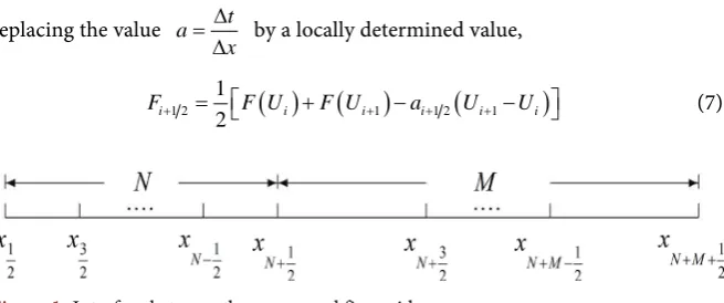
For ease of presentation, we consider the case of mesh refinement by a factor

θ_{. Figure 1 shows a grid consists of two uniform subgrids and the factor}

2

θ = _{. Suppose the problem is on the physical domain}

[ ]

subdi-vided into cells 1,, N, N+1,,N M+ with 1 2

x =a and 1 2

N M

x b

+ + = , so that

1 N

b a

x x

N Mθ

− ∆ = = ∆ =

+

 and N 1 N M

b a

x x

N Mθθ

+ +

− ∆ = = ∆ =

+

 . Apparently,

the interface between the coarse and fine grids is located at 1 2

N

x + .

3. Numerical Methods

The equations presented in the previous section will be solved using first order accurate LLF [7] method. The scheme for solving Equations (1)-(5) can be writ-ten in the form

(

)

1

1 2 1 2 ,

n n n n

i i i i

t

U U F F

x

+

+ −

∆

= − −

∆ (6)

where 1 2

n j

F+ is the numerical flux function at the interface between cells i

and i+1 at time level n. Depending on the choice of the numerical flux

for-mula, Equation (6) is referred to as LLF scheme.

LLF scheme is the improved version of the classical Lax-Friedrichs scheme by replacing the value a t

x

∆ =

∆ by a locally determined value,

( )

(

)

(

)

1 2 1 1 2 1

1 2

i i i i i i

F+ = F U +F U+ −a+ U+ −U  (7)

where ai+1 2=max

(

( ) (

)

)

4. Numerical Result

4.1. Advection Equation

Firstly, advection Equation (1) is considered on a non-uniform grid which is composed of two uniform subgrids with initial condition

( )

, 0

0, if 1 1.

x u x x − ≤ ≤ −  =  _{− ≤ ≤} 

The ratio between the coarse and fine grids is θ =2, and the interface in the

physics domain is located at x=0. The boundary of domain a= −2, b=1,

and the number of cell N=200, M =200. Obviously, the discontinuity will

arrive the interface when t=1 and wholly pass through it when t=1.5.

For the linear advection equation, LLF scheme reduces to upwind scheme. The solutions to advection equation can be seen in Figure 2. From this figure, we find that the solution has monotone profile as expected and no oscillation can be observed around x=0.

4.2. Inviscid Burgers Equation

The second example is the inviscid Burgers Equation (2) subject to the initial data

( )

0, if 1 1.

x u x x − ≤ ≤ −  =  _{− ≤ ≤} 

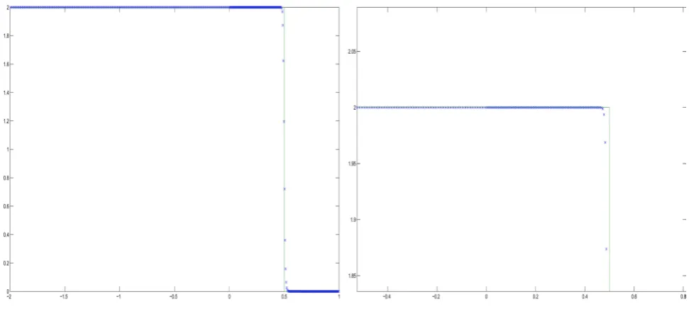
The solution propagates to the right with shock speed s=1. Figure 3 shows

the solution at t=1.5, and the shocks pass through the interface at t=1. The

zoomed version around x=0 is shown in Figure 3. As in the previous

prob-lem, LLF scheme shows monotone solutions which are similar to the solutions on the uniform grids.

4.3. Shallow Water Equations

Consider the shallow water equations (3) with the piecewise-constant initial conditions

( )

( )

1, if 0 5,

x

h x u x

x

− ≤ ≤ 

=_ =

≤ ≤

 (8)

This is a special case of the Riemann problem in which ul =ur =0, and is

called the dam-break problem because it models what happens if a dam separat-ing two levels of water bursts at time t=0. This is the shallow water equivalent

of the shock tube problem of gas dynamics.

Note that the Jacobian matrix

F u

′

( )

( )

0 1

. 2 F u

u gh u

 

′ _{=  }

− +

 

Figure 2. Left: numerical solution at t=1.5 with LLF scheme. Right: zoomed region around the interface between the coarse and

fine grids.

Figure 3. Left: numerical solution of Burgers equation at t=1.5 with LLF scheme. Right: zoomed region around the interface 0

x= between the coarse and fine grids.

1 2

, ,

u gh u gh

λ = − λ = +

with the corresponding eigenvectors

1 1 2 1

, .

r r

u gh u gh

   

=  = 

− +

   

   

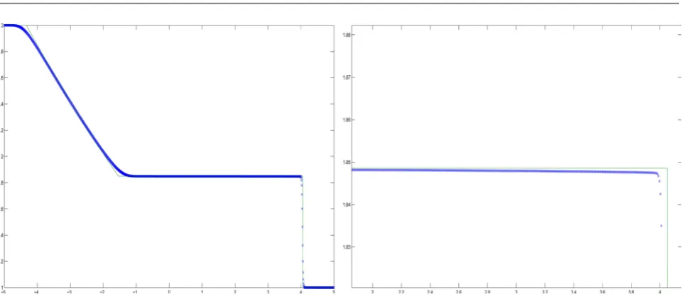
Firstly, a uniform grid is considered. Figure 4 shows the structure of solution of this Riemann problem. Note that the shallow water equations are a system of two equations, and so the Riemann solutions generally contain two waves. For this initial-value problem (3) (8), these always consist of one 1-rarefaction wave on the left and one 2-shock on the right with shock speed s≈1.6226. In this

case, we find that the solutions behave well and no postshock oscillation is in-troduced.

Figure 4. Left: solution of the dam-break Riemann problem for the shallow water equations with ul=ur=0 on uniform grids;

Right: zoomed version around x=3.

loci and integral curves. The Hugoniot curves correspond to the 1-shock and 2-shock are

(

)

2 l

l l

l

h

g h

hu u h h h

h h

  = − _ − _ −

 

and

(

)

2 r

r r

r

h

g h

hu u h h h

h h

  = + _ − _ −

 

respectively.

The integral curves correspond to 1-rarefaction and 2-rarefaction waves are

(

)

2

l l

hu=hu + h gh − gh

and

(

)

2

r r

hu=hu − h gh − gh

respectively.

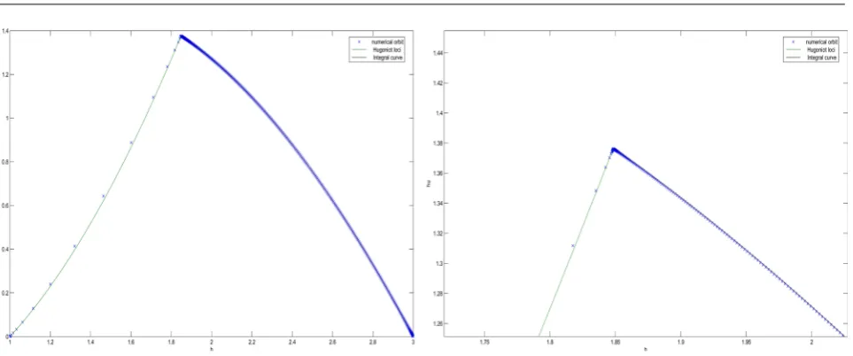
As shown in previous paragraph, the solution of this initial-value problem contains both shock and rarefaction. So, Hugoniot and integral curves originate from the left state Ur and right state Ul, and the intersection of them is

in-termediate state Um. Figure 5 shows that numerical solution by LLF scheme

almost lies on the Hugoniot and integral curves.

In Figure 6, physics domain

[

]

[

]

and

[ ]

De-note the length of the cells on interval

[

]

[ ]

respectively. Figure 6 shows the solution on nonuniform grids with ∆ ∆ =xl xr 2

at t=2.5. Amplifying the figure around interface at x=3, an obvious

Figure 5. Left: Hugoniot loci and integral curve of the eigenvector 1

r for the shallow water equations in the state space

(

)

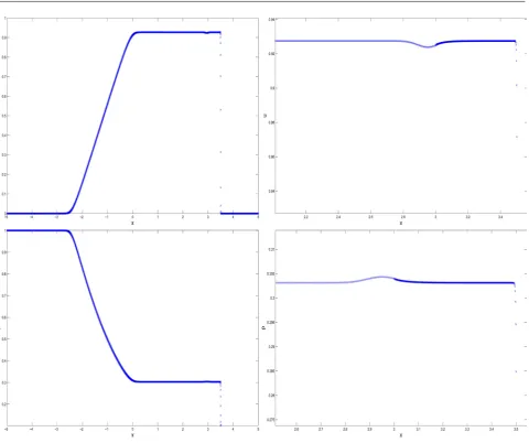
Figure 6. Solution of the dam-break Riemann problem for the shallow water equations with nonuniform grids which consist of two uniform grids with ∆xl ∆ =xr 2.

after it pass through the interface. The oscillation is the wave that arose from the initial discontinuity at x=3 when the shocks pass the interface.

A interesting phenomenon can be observed in Figure 7. The hump (oscilla-tion) in Figure 6 changes into dip if we shift ∆xl ∆xr from 2 into 0.5. Note

that the hump and dip both belong to acoustic wave moving at speed

0.6148

m m

u −c ≈ − , where cm = ghm .

Note that, for the shallow water equations, the function of 1-Riemann inva-riant and 2-Riemann invainva-riant are

1

2

w = +u gh

and

2

2

w = −u gh

respectively.

curve of r1. Similarly, the value of 2-Riemann invariant is constant along any

integral curve of 2

r . We find that the acoustic wave (oscillation behind the shock) takes the same value as 1-rarefaction wave for 1-Riemann invariant.

Figure 9 shows Hugoniot, integral curves and numerical orbit in state space on nonuniform grids. Note that the numerical orbit deviating the integral curve in Figure 9 is due to the departure between numerical solution and exact solu-tion at the left of the shock. In addisolu-tion, a redundant tip appears in this figure which is different from the distribution of numerical orbit in Figure 5.

4.4. 1D Euler Equations

Euler equations of gas dynamics is discussed in this section. We test the post-shock oscillations with initial data

(

) (

₍

)

₎

0.125, 0, 0.1 , if 0.

x v p

x

ρ _{= } ≤ >

 (9)

This is a well known test problem proposed by Sod [9]. The physical domain

Figure 7. Solution of the dam-break Riemann problem for the shallow water equations with nonuniform grids which consist of two uniform grids with ∆ ∆ =x_l x_r 0.5.

Figure 9. Left: Hugoniot loci and integral curve of the eigenvector 1

r for the shallow water equations in the state space

(

)

Right: zoomed version.

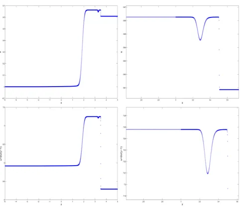
Figure 10. Numerical solution of Sod problem on nonuniform grids at t=2.0.

[

]

[

]

[ ]

Except for the first and third characteristic fields are genuinely nonlinear which have similar behavior to the two characteristic fields in the shallow water equations, the second field is linearly degeneration. So, the solution to Riemann problem for Euler problem typically has two nonlinear waves and a contact dis-continuity.

Figure 10 shows the numerical solution on nonuniform grids with

4

l r

x x

∆ ∆ = . The shock has already passed through the interface at t=2.0, and

two humps arise near x=3. This is different from what we observed in shallow

From Figure 10, we find that two waves propagate with different direction. Note that these two waves are different from some nonphysical oscillations. The left wave propagate to the left with the speed * *

0.3367

u −c = − , and the left

wave propagate to the other direction with the speed *

0.9275

u = , where

aste-risk denotes intermediate state and * * *

r

c = γp ρ . In addition, the amplitude

of vibration is decided by the ratio ∆xl ∆xr. The bigger ratio between the coarse

and fine grids, the bigger amplitude the postshock will have.

For this initial value problem, all of the Riemann invariants for a polytropic ideal gas are summarized below:

2 1-Riemann invariants, , ,

1

2-Riemann invariants, , ,

2 3-Riemann invariant, .

1 c s u

u p

c u

γ

γ

+ −

− −

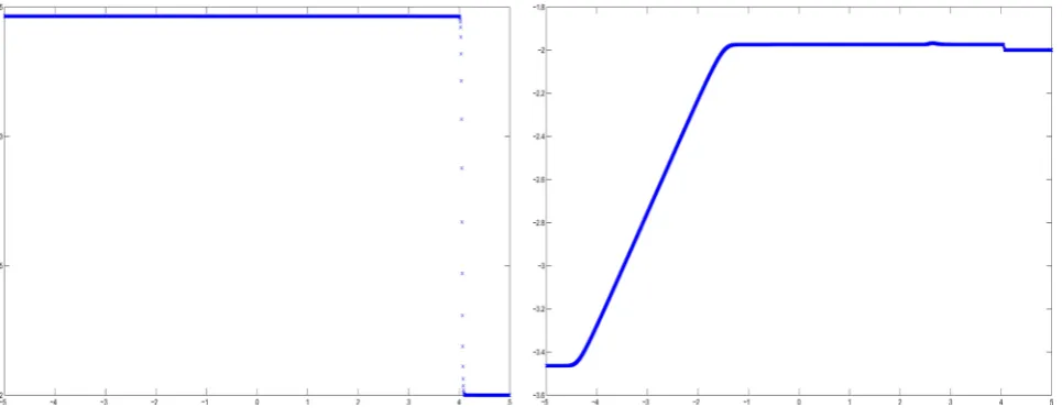
Figure 11 shows the 1-Riemann invariants for this initial value problem. We

Figure 12. 2-Riemann invariants.

find that the 1-Riemann invariants are constant across the rarefaction and the left wave which generate from x=3, and only one oscillation was left.

Similar-ly, Figure 12 shows the 2-Riemann invariants which are constant across the second oscillation at the right of x=3. And 3-Riemann invariant is given in

Figure 13. From these three figures, the oscillations behind the shock behave similarly to the rarefaction for Riemann invariants.

4.5. 2D Euler Equations

The last example is 2D Euler equations (5), with initial data

(

)

(

)

(

)

(

)

(

)

1.1, 0.0, 0.0,1.1 , if 0.5, 0.5,

0.5065, 08939, 0.0, 0.35 , if 0.5, 0.5,

, , ,

1.1, 0.8939, 0.8939,1.1 , if 0.5, 0.5,

0.5065, 0.0, 0.8939, 0.35 , if 0.5, 0.5,

x y

x y

u v p

x y

x y

ρ

 > >

 _{< >}



=  _{< <} 

 _{> <}



(10)

shock across the interface.

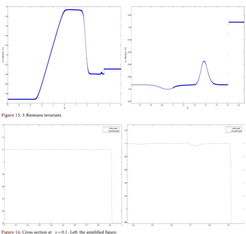
Figure 14 shows the cross-sectional solution at x=0.1. One solution on

uni-form grids and another solution on nonuniuni-form grids are shown in this figure. The obvious difference between these two solutions is that two additional humps appear in the solution under nonuniform grids. This phenomenon is similar to what appear in the previous nonlinear system.

5. Conclusion

The postshock oscillations appeared in the nonlinear system has been elucidated numerically. We found that these oscillations would not appear in the nonlinear scalar equation and linear equations system. Although all the numerical results were computed with LLF method, these oscillations also appeared with other schemes, such as Godunov, Roe schemes and so on. So the postshock oscillations

Figure 13. 3-Riemann invariant.

have nothing to do with the specific methods which are used to compute solu-tion on nonuniform grids. In addisolu-tion, this kind of oscillasolu-tions is different from those nonphysical oscillations arose near the shock, and they are similar to those emerge behind the slow-moving shocks which can be found in [5][6].

Acknowledgements

This work was supported by the National Natural Science Foundation of China (No. 11501238), Natural Science Foundation of Guangdong Province (No. 2012A030313119) and Supported by the Major Project Foundation of Guang-dong Province Education Department (No. 2014KZDXM070).

References

[1] Berger, M.J. and Colella, P. (1989) Local Adaptive Mesh Refinement for Shock Hy-drodynamics. Journal of Computational Physics, 82, 64-84.

https://doi.org/10.1016/0021-9991(89)90035-1

[2] Berger, M.J. and Oliger, J. (1984) Adaptive Mesh Refinement for Hyperbolic Partial Differential Equations. Journal of Computational Physics, 53, 484-512.

https://doi.org/10.1016/0021-9991(84)90073-1

[3] Huang, W., Ren, Y. and Russell, R.D. (1994) Moving Mesh Partial Differential Equ-ations (MMPDES) Based on the Equidistribution Principle. SIAM Journal on Nu-merical Analysis, 31, 709-730. https://doi.org/10.1137/0731038

[4] Stockie, J.M., Mackenzie, J.A. and Russell, R.D. (2001) A Moving Mesh Method for One-Dimensional Hyperbolic Conservation Laws. SIAM Journal on Scientific Com-puting, 22, 1791-1813. https://doi.org/10.1137/S1064827599364428

[5] Roberts, T.W. (1990) The Behavior of Flux Difference Splitting Schemes near Slow-ly Moving Shock Waves. Journal of Computational Physics, 90, 141-160.

https://doi.org/10.1016/0021-9991(90)90200-K

[6] Arora, M. and Roe, P.L. (1997) On Postshock Oscillations Due to Shock Capturing Schemes in Unsteady Flows. Journal of Computational Physics, 130, 1-24.

https://doi.org/10.1006/jcph.1996.5534

[7] Rusanov, V.V. (1962) The Calculation of the Interaction of Non-Stationary Shock Waves and Obstacles. USSR Computational Mathematics and Mathematical Phys-ics, 1, 304-320.

[8] Leveque, R.J. (2002) Finite Volume Methods for Hyperbolic Problems. Cambridge University Press, Cambridge. https://doi.org/10.1017/CBO9780511791253

[9] Sod, G.A. (1978) A Survey of Several Finite Difference Methods for Systems of Nonlinear Hyperbolic Conservation Laws. Journal of Computational Physics, 107, 1-31. https://doi.org/10.1016/0021-9991(78)90023-2

[10] Lax, P.D. and Liu, X.D. (1998) Solutions of Two-Dimensional Riemann Problems of Gas Dynamics by Positive Schemes. SIAM Journal on Scientific Computing, 19, 319-340. https://doi.org/10.1137/S1064827595291819

[11] Schulz-Rinne, C.W., Collins, J.P. and Glaz, H.M. (1993) Numerical Solution of the Riemann Problems for Two-Dimensional Gas Dynamics. SIAM Journal on Scien-tific Computing, 14, 1394-1414. https://doi.org/10.1137/0914082

Submit or recommend next manuscript to SCIRP and we will provide best service for you:

Accepting pre-submission inquiries through Email, Facebook, LinkedIn, Twitter, etc. A wide selection of journals (inclusive of 9 subjects, more than 200 journals)

Providing 24-hour high-quality service User-friendly online submission system Fair and swift peer-review system

Efficient typesetting and proofreading procedure

Display of the result of downloads and visits, as well as the number of cited articles Maximum dissemination of your research work

Submit your manuscript at: http://papersubmission.scirp.org/