Serial default and debt renegotiation

Munich Personal RePEc Archive

Serial default and debt renegotiation

Asonuma, Tamon

International Monetary Fund

2 April 2012

Online at

https://mpra.ub.uni-muenchen.de/55139/

Serial Default and Debt Renegotiation

Tamon Asonumay

International Monetary Fund

April 2, 2012

Abstract

Emerging countries that have defaulted on their debt repayment obligations in the past are

more likely to default again in the future than are non-defaulters even with the same

debt-to-GDP ratio. This paper explains this stylized fact within a dynamic stochastic general equilibrium

framework by explicitly modeling renegotiations between a defaulting country and its creditors.

The quantitative analysis of the model reveals that the equilibrium probability of default for a

given debt-to-GDP level is weakly increasing with the number of past defaults, consistent with

empirical observations. The equilibrium of the model also accords with an additional observed

fact: a country for which default terms require less than a 100 percent recovery rate tends to pay

a higher rate of return (relative to a risk-free rate) on subsequently issued debt than do defaulting

countries that agree to a full recovery rate.

JEL Classi…cation Codes: E43; F32; F34; G12

Key words: Serial default; Debt renegotiation; Past credit history; Recovery rates; Interest

spreads

I am indebted to Marianne Baxter, Francois Gourio, Laurence Kotliko¤ and Adrien Verdelhan for guidance and support. I am also grateful to Christoph Trebesch for kindly providing the data. I thank Jochen Andritzky, Ran Bi, Charles Blitzer, Marcos Chamon, Bertrand C. Gruss, Juan Carlos Hatchondo, Allison Holland, Cosmin Ilut, Jun Il Kim, Hanno Lustig, Stephen Morris, Romain Ranciere, Guillem Riambau, Leena Rudanko, Georg Strasser, Cedric Tille, Christoph Trebesch, Siew Ling Yew, Vivian Yue and Mark Wright for useful comments and suggestions as well as seminar participants at the IMF RES, INS, AFR, the 2009 Midwest Theory, the 2009 Midwest Macroeconomic Meeting, the 2009 North American Summer Meeting of Econometric Society, the 2009 European Economic Association, the 2010 American Economic Association, the 2010 Society of Economic Dynamics, Modeling Economic Dynamics, BC-BU Green Line Macro Meeting, Berlin Conference on Sovereign Debt, Boston U., GRIPS, Keio U., Osaka U., Banco de Espana, Durham Business School, Birmingham Business School, Bank of Japan, Halle Economic Research Institute, Geneva Graduate Institute, Dutch Central Bank, CERDI, and LUISS. Additional thanks go to Andrew Ellis and Jeremy Smith for editorial suggestions and Brian Moon for research assistance. An early version of this paper has been circulated with the title "Sovereign default and renegotiation: recovery rates, interest spreads and credit history". All remaining errors are my own. Any views expressed in this paper are those of the author and do not re‡ect any views of the International Monetary Fund.

1

Introduction

Emerging countries that have defaulted on their debt repayment obligations in the past are more likely

to default again in the future than are non-defaulters with the same debt-to-GDP ratio. This paper

explains this stylized fact within a dynamic stochastic general equilibrium framework that explicitly

models renegotiations between a defaulting country and its creditors. Speci…cally, the model extends

the existing literature by allowing the defaulter and creditors to bargain not just over recovery rates,

but also over the rate of return o¤ered on newly-issued debt. Quantitative analysis of the model

reveals that the equilibrium probability of default for a given debt-to-GDP level is weakly increasing

with the number of past defaults, consistent with empirical observations. The equilibrium of the

model also accords with an additional observed trend: a country for which default terms require less

than a 100 percent recovery rate tend to pay a higher rate of return (relative to a risk-free rate) on

debt that is issued subsequently than do defaulting countries that agree to a full recovery rate. These

…ndings are robust to extensions that allow the renegotiation outcome to be modeled more ‡exibly.

This paper deals with endogenous debt renegotiation after default in a standard dynamic model of

defaultable debt. The renegotiation process involves Nash bargaining between the defaulting debtor

and creditors over both the recovery rate and increases in rates of return on new debt. Evidence

suggests that the spread between the rate of return on new debt and the risk-free rate increases after

default more for defaulters that pay less than a full recovery rate than for defaulters that agree to repay

all of the defaulted debt (i.e. a 100 percent recovery rate). Thus, it appears that, at least implicitly,

a country that defaults negotiates with its creditors both over recovery rates and over future rates

of return. This re‡ects a trade-o¤ for defaulting country: the defaulted debt can be repaid in the

present at a high short-run cost in return for only a small or even negligible deterioration in long-term

credit condition; or the short-run bene…t of repaying the debt only partially will be o¤set by having

to pay lenders a higher rate of return on future issuances. The trade-o¤ for creditors is symmetric: if

they are not appeased by a full recovery of funds in the short term, they can attempt to recoup their

losses by demanding higher rates of return for holding the country’s bonds in the future.

The present paper seeks to incorporate these trade-o¤s facing the debtor and creditors during

renegotiations following defaults. In the model, the endogenously-determined terms of renegotiations

increases in yield spreads. An emerging country that defaults once therefore pays a penalty either

through a large recovery rate in the short term or through higher borrowing costs in the long term.

If it chooses to repay less than full recovery rates, it will face high borrowing costs, which lead

to increase the risks that the country will default again in the future. This mechanism drives the

equilibrium serial default behavior in the model, and it is a plausible explanation of the pattern of

repeat defaults observed in the data. Hence, the model is able to jointly explain both stylized facts

of debt renegotiations and repeat defaults.

We embed the debt renegotiation in a dynamic sovereign debt model with endogenous defaults

where an emerging country is subject to exogenous income shocks. This part of the model builds on

recent quantitative analysis of sovereign debt such as Aguiar and Gopinath (2006), Arellano (2008)

and Tomz and Wright (2007) which are based on classical setup of Eaton and Gersovitz (1981). At the

renegotiation, creditors and defaulting country bargain over increases in rate of return on new debt

together with recovery rates. Outcomes of the renegotiation represent trade-o¤s of both defaulting

country and creditors, as indicated above. Total spread between the rate of return on new debt and

the risk-free rate, incorporates not only the probability of future default but also impacts on increases

in rate of return on new debt agreed at the past renegotiations.

Our paper is most closely related with Yue (2010), in which a dynamic model of defaultable debt

is argumented with an endogenous treatment of debt renegotiation after default. Our model di¤ers

from her model in that we incorporate the e¤ects of increases in rate of return on new debt. At the

renegotiation, both parties bargain not only over recovery rates, but also over increases in rate of

return on new debt. Therefore, its credit condition, i.e. borrowing cost of the country after re-entry to

the market, depends on how much the country pays at the debt renegotiation. Increase in borrowing

costs accompanied by repaying the debt only partially will lead to increase future default probability.

In special case where the country always repays in full the level of defaulted debt, increases in rate

of return on new debt will be close to zero. As impacts of additional default premia are totally

negligible, results will be quite similar to ones in Yue (2010).

The rest of the paper is organized as follows. Section 2 reviews two strands of literature. Section

3 overviews stylized facts of debt negotiations and serial defaults. We provide our stochastic dynamic

general equilibrium model in Section 4. We de…ne recursive equilibrium of the model in Section

Section 7. A short conclusion summarizes the discussion. The computation algorithm is provided in

Appendix A.

2

Literature Review

This paper is related to the literature of serial default. Reinhart, Rogo¤ and Savastano (2003) and

Reinhart and Rogo¤ (2005) both advocate the role of past credit history in debt intolerance. On

con-trary, Eichengreen, Hausmann, and Panizza (2003) show that countries with "original sin", inability

to issue bonds in their domestic currencies, must pay an additional risk premium when they borrow,

increasing their solvency risks since the …nancial market knows this inability is a source of …nancial

fragility. However, none provides economic models describing how weak credit history or "original

sin" features are associated with serial defaults. With stochastic dynamic model, Kovrijnykh and

Szentes (2007) explain the equilibrium default cycles, but they do not derive any relation between

de-fault occurrences and outcomes of negotiations. This paper improves these papers by explaining how

outcomes of current debt renegotiation, such as additional spread premia, lead to higher probability

of next default in future.

The other strand of literature models the sovereign default and renegotiation as a game between

a sovereign debtor and its creditors.1 _{Yue (2010) treats debt renegotiation process using a}

one-round Nash bargaining game. Moreover, Bai and Zhang (2010), Benjamin and Wright (2009) and Bi

(2008) presume a multi-round bargaining to analyze delay in renegotiation. Benjamin and Wright

(2009) assume that debtor and representative creditor randomly alternate in their ability to propose

a bargaining outcome with changes in the probability of making future proposals serving to capture

changes in bargaining power, while Bi (2008) supposes that lenders have an option to "pass" proposing

to the debtor. Bai and Zhang (2010) focus on the role of information friction which generates the

delay. Furthermore, Pitchford and Wright (2007) regard multi-creditor renegotiation process as a

series of bilateral bargaining games to explain delays in renegotiation. Similarly, Kovrijnykh and

Szentes (2007) also study multi-creditor renegotiation and makes the time of exclusion from the

…nancial market endogenously and potentially long. Our paper di¤ers from this literature in that

1_{Our borrowing environment, besides the debt renegotiation, is a version of the Eaton and Gersovitz (1981) model of}

we concentrate on the observed pattern that lower recovery rates at the renegotiation are highly

associated with larger increases in yield spreads.2

Lastly, our empirical …nding is linked to studies analyzing the impacts of past defaults on future

spreads. Ozler (1993) …nds that past defaulters had to pay a premium on the interest rate for the

sovereign debt issued in the 1970s and defaults previous to 1930 did not a¤ect the premium paid but

defaults after that did a¤ect it. In a similar context, Ozler (1992) empirically shows that borrower’s

repeated experience in the market contributes signi…cantly to the variation of spreads. Cantor and

Packer also con…rm that sovereign yields tend to rise as sovereign has a bad default history.3 On

the contrary, Lindert and Morton (1989) focusing on borrowing experience in late 1970s, …nd no

evidence that defaulters were punished by creditors through higher interest rates on new loans. What

is distinctive in our paper relative to previous work is that we analyze the deterioration of long-term

borrowing in the short window after the renegotiations on bonds during 1986-2007 and how it di¤ers

in terms of agreed recovery rates.

3

Stylized facts

Evidence of serial defaults re‡ects that past defaulters are more likely to default in the future than

are non-defaulters given the debt-to-GDP ratio. Moreover, from recent debt renegotiation episodes,

we observe that lower recovery rates at the renegotiation are highly associated with larger increases

in yield spreads between the rate of return on new debt and the risk-free rate.

3.1 Evidence on serial defaults

In this subsection, we cover stylized facts of serial defaults, especially some features di¤ering by

countries’ history of defaults.

2_{We assume that debt renegotiation takes place only once for each default.}

3_{Trebesch (2009) indicates that unilateral, aggressive sovereign debt policies lead to a stronger decline in corporate}

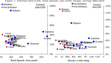
Figure 1: External debt/GDP, bond spreads, and credit ratings, average 2005-2010

Source: Bloomberg, Datastream, De Paoli, Hoggarth and Saporta (2006), Haver, IMF WB

Quarterly External Debt Statistics, IMF World Economic Outlook and Moody’s.

Figure 1 reports external debt-to-GDP ratio, bond spreads and credit ratings. Bond spreads

of past defaulters are higher than those of non-defaulters given external debt-to-GDP ratio. Past

defaulters tend to su¤er higher spreads on the newly issued bonds in the future after default, even

if they have the same level of foreign debt relative to GDP as before. Similarly, past defaulters have

lower credit ratings than non-defaulters, re‡ecting higher default probability.

Moreover, Reinhart, Rogo¤ and Savastano (2003) show that countries with a weak credit history

may become more vulnerable even at much lower levels of external debt, relative to countries with a

sound credit history. Table 1 illustrates predicted Institutional Investor ratings and debt intolerance

regions for Argentina and Malaysia.4

[Insert Table 1 here]

4_{In order to address this point, Reinhart, Rogo¤ and Savastano (2003) use the estimated coe¢cients from the}

It is apparent that precarious debt intolerance situation of Argentina is more severe than one

of Malaysia.5 Since Argentina is representative of many countries with a weak credit history and

Malaysia is representative of countries with a sound credit history, this result re‡ects that the debt

thresholds of countries with a weak credit history are lower than that of countries with a sound credit

history. In other words, the default probability of countries with a weak credit history is higher than

one of countries with a sound credit history, given the same level of debt-to-GNP.

In addition, Reinhart, Rogo¤ and Savastano (2003) report that defaulters repeat defaults or

restructurings in short periods: emerging countries with at least one external default or restructuring

since 1824, have experienced 5.2 defaults or restructurings in average as shown in Table 2.

[Insert Table 2 here]

3.2 Recent sovereign debt renegotiations

We start with an overview of recent debt renegotiation episodes. Table 3 summarizes 15 cases of

expost-default and preemptive restructurings in the ten years from 1998 to 2007.6 We present default

year, defaulted debts, recovery rates, and increases in interest spreads for each episode. One feature

which stands out is that recovery rates vary depending on the cases.

[Insert Table 3 here]

Furthermore, Figure 2 displays recovery rates and increases in spreads for 35 sovereign debt

renegotiation episodes during 1986-2007.78

5_{Argentina only remains in the relatively safe "region 1" as long as its external debt is below 15 percent of GNP,}

whereas Malaysia stays in "region1" up to a debt-to-GNP ratio of 30 percent, and it is still in the relatively safe "region

2" with a debt of 35 percent of GNP.

6_{We exclude the cases of swap agreements and delay in payment such as Venezuela in 1995, 1998 and 2005, Peru in}

2000 and Paraguay in 2003.

7_{For 6 cases such as Argentina 2001, Ecuador 1999, Pakistan, Russia 1998, Ukraine 1998, Uruguay 2003, we use}

recovery rates in Sturzenegger and Zettlemeyer (2008). Recovery rates for Grenada, Dominican Rep.2005 and Belize are from Bedford, Penalver and Salmon (2005). The remaining cases are based on Benjamin and Wright (2009).

8_{Sturzenegger and Zettelmeyer (2006, 2008) de…ne recovery rates as the market value of the new instruments, plus}

Figure 2: Recovery rates and increases in spreads for recent debt renegotiations

Source: Bedford, Penalver and Salmon (2005), Benjamin and Wright (2009), Datastream, and Sturzenegger

and Zettelmeyer (2006 and 2008)

We focus only on expost-default and preemptive renegotiation episodes in the sample periods,

and we exclude examples of delays in payment such as Paraguay in 2003, and Venezuela in 1995,

1998, 2005, and swap agreement for Peru in 2000. We de…ne "increase in spreads" as the di¤erence

in spreads between the time of renegotiation and one year before the renegotiation.910 The …tted

line is obtained by regressing recovery rates on increases in spreads controlling for actual detrended

GDP and political indicators as indicated in the third column of Table 4. This negative relationship

is robust even controlling for debt/GDP ratio and omitting an outlier case of Russia 1998 shown

9_{The bond spreads data are from the J.P. Morgan’s Emerging Markets Bond Index Global (EMBIG) data for}

respective countries. Included in the EMBI Global are U.S.-dollar-denominated Brady bonds, Eurobonds, traded loans, and local market debt instruments issued by sovereign and quasi-sovereign entities. The spreads are computed as an arithmetic, market capitalization-weighte average of bond spreads over U.S. treasury bonds of comparable duration.

1 0_{According to J.P. Morgan (1999), a new issue that meets the EMBI Global’s admission requirements is added to the}

in the fourth and …fth columns respectively.11 These results re‡ect that lower recovery rates at the

renegotiation are associated with larger increases in yield spreads between the rates of return on new

debt and the risk-free rate. This presents a trade-o¤ for defaulting countries; if the countries recover

a larger fraction of debt at the renegotiations, long-term borrowing costs will be smaller. At the same

time, we can interpret it as a trade-o¤ of creditors. If the creditors receive payments for only a small

fraction of defaulted debt, they can recoup their losses by demanding higher rates of return for the

newly issued bonds.

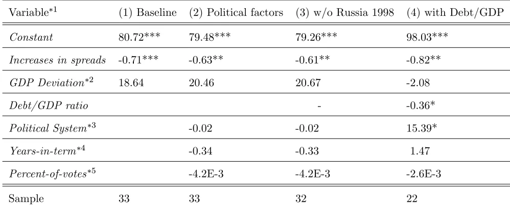
Table 4: Regression results

Variable 1 (1) Baseline (2) Political factors (3) w/o Russia 1998 (4) with Debt/GDP

Constant 80.72*** 79.48*** 79.26*** 98.03***

Increases in spreads -0.71*** -0.63** -0.61** -0.82**

GDP Deviation 2 18.64 20.46 20.67 -2.08

Debt/GDP ratio - -0.36*

Political System 3 _{-0.02 -0.02 15.39*}

Years-in-term 4 -0.34 -0.33 1.47

Percent-of-votes 5 _{-4.2E-3 -4.2E-3 -2.6E-3}

Sample 33 33 32 22

Source: Bedford, Penalver and Salmon (2005), Benjamin and Wright (2009), Datastream, Sturzenegger and

Zettelmeyer (2006 and 2008), Reinhart and Rogo¤ (2010), and World Bank The Database for Political

Institutions (PDI). Note: Standard errors are in parentheses. ***, **, * show signi…cance at 1, 5, and 10

percent levels respectively. 1: All regression results are based on least square estimations. 2: GDP deviation

from the trend is a percentage deviation from the trend obtained by applying the Hodrick-Prescott (H-P)

…lter. 3: "Political system" indicator is di¤erenciated by parliamentary, assembly-elected president, and

presidential ststems. 4: "Years-in-term" indicator de…nes years left in current term. 5: "Percent-of-votes"

indicator speci…es percentages of votes the current president got in the 1st round of election.

1 1_{When we de…ne "increase in spreads" for 2-year window, such as the di¤erence between one year before and after}

4

Model environment

The basic structure of the model follows previous work that extends the model of sovereign default

by Eaton and Gersovitz (1981) and applies its quantitative analysis. Among these studies, the closest

reference to our paper is Yue (2010). The distinctive feature in our model with respect to her model

is that we introduce e¤ects of increases in rate of return on new debt after the re-entry to the market.

Since both recovery rates and increases in rate of return on new debt are determined endogenously,

how much the country pays at the renegotiation will a¤ect its credit condition in the future, i.e.

borrowing costs of the country after re-entry to the market, which will have impacts on default

probability.12

4.1 General points

The model analyzes sovereign default and negotiation in a stochastic dynamic equilibrium model. We

consider a risk-averse country that can’t a¤ect world risk-free interest rate. The country’s preference

is given by following utility function:

E0 1 X

t=0

t_u(c t)

where 0 < <1 is a discount factor, ct denotes consumption in period t, and u(:) is its one-period

utility function, which is continuous, strictly increasing and strictly concave and satis…es the Inada

conditions. A discount factor re‡ects both pure time preference and probability that the current

sovereignty will survive into next period.

In each period, the country starts with its credit history ht, which satis…es ht 2 H where

H = [0;1;2; :::; hmax]. The credit history expresses number of debt renegotiations the country has

experienced in the past.13 The reason why we assume multi-state credit history rather than

two-state credit history as in Yue (2010) is to analyze how the outcomes of past debt renegotiations

associated with defaults a¤ect the probability of next default. Moreover, we assume that the credit

1 2_{On contrary, Yue (2010) has not taken into account impacts of increases in rate of return on new debt. In her model,}

both parties negotiate over only recovery rate after default. The reason why e¤ects of increases in rate of return on new debt are missing in her model is that the country’s credit condition will always return to the same level irrelevant to recovery rate which is determined at the renegotiation.

1 3_{The model simply distinguishes h}

t = 0 andht >0 as the non-default history and defaulting history, not as the

history reverts with exogenous probability conditional on that the country chooses to pay the spread

returns after defaults.14

The country receives an exogenous income shockyt. Income shock (yt) is stochastic, drawn from

a compact set Y = [ymin; ymax] R+. (yt+1jyt) is the probability distribution of a shock yt+1

conditional on previous realization yt.

There is an in…nite number of investors who are risk-neutral and behave competitively in the

international capital market. They have perfect information on the country’s assets, credit history,

income shocks and additional spread premia agreed to at previous debt renegotiation. We also

assume that they can borrow or lend as much as needed at a constant risk-free interest rate (r) in the

market. Since they are symmetric and similarly ranked, we can interpret them as "a representative

investor" lending money to the country. The country borrows the money from the same representative

investor though bond exchanges even after it defaults.15 _{As investors are able to collude at the debt}

renegotaition, "a representative investor" has a bargaining power at the renegotiation in order to

impose higher spreads on future bonds, though its bargaining power is low compared to that of

country.16 Moreover, we assume that all the investors behave in the same manner: they all lend the

money to the country every time the country issues bonds, and there is no sub-group of investors

who behave di¤erently from the majority of investors such as they still lend money to the country

even if the country defaults and refuse to negotiate with the majority of investors.17

The international capital market is incomplete. The country and foreign investors can borrow

and lend only via one-period zero-coupon bonds where bt+1 denotes amount of bonds to be repaid

next period. When the country purchases bonds, bt+1 >0, and when it issues new bonds, bt+1 <0.

1 4_{Following the consumer defaults as in Chatterjee et al (2007), we assume that the record of the recent default}

remains on the country’s credit history for only a …nite number of years.

1 5_{The country negotiates wtih the creditors who hold its debts and the creditors receive the recovered debts as in}

current model. Thus, it is true that the country borrows again from the same creditors. While in the reality, there exists the secondary markets where the creditors can sell and purchase the exchanged bonds, the current model abstracts this feature.

1 6_{In usual debt restructurings, the bond holders organize a committee, which conduct research on the soverign and}

consolidate creditors’ view to faciliate the discussion. Given the restructuring plan proposed by the soverign, all creditors vote on it. If a critical mass of the creditor approve, the proposal is passed and …nalized. Otherwise, the government has to revise the proposal until it passes. In order to smooth the renegotiation, the committee plays an important role to re‡ect the creditors’ view on the sovereign’s proposal. Thus, it is identical to say that a committee has a barganing power, but it is relatively low as the committee has a di¢culity to consolidate views across investors. Rie¤el (2003) provides description of sovereign debt renegotiation.

1 7_{It is true that the current model abstracts elements of entry of new creditors and existance of secondary markets.}

The set of amount of bonds is B = [bmin; bmax] R wherebmin 0 bmax. The upper bound is the

highest level of assets that the country can accumulate and the lower bound is the highest level of

debts that the country can hold. We assumeq(bt+1; ht; yt) is the price of a bond with asset position

(bt+1), credit history (ht), and income level (yt). The bond price will be determined in equilibrium.

We assume that foreign investors always commit to repay their debt. However, the country is

free to decide whether to repay its debt or to default. If the country chooses to repay its debt, it will

preserve access to the international capital market next period.

If the country chooses not to pay its debt, it is subject to both exclusion from the international

capital markets and direct output cost.1819 When a default occurs, the country and foreign investors

negotiate reduction of unpaid debt via Nash bargaining. At the renegotiation, both recovery rates

and additional spread premia on the newly issued bonds are agreed to by both parties.20 The country

regains access to the market after excluded from the market a short period, but the country’s credit

history records the current debt renegotiation.21 _{In order to avoid permanent exclusion from the}

international capital market, the country has an incentive to negotiate over haircut rates (recovery

rates) and additional default premia. From foreign investors’ point of view, Foreign investors want to

maximize the payment from recovered debt and spread returns on newly issued bonds after default,

so they are also willing to negotiate over reduction of unpaid debt.

All the information on the country’s asset, credit history, and income realization is perfect.22

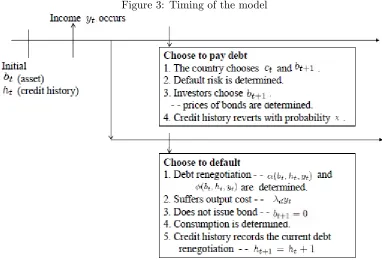
4.2 Timing of the model

Timing of decisions within each period is summarized in Figure 3.

1 8_{There are several estimates for output loss at the time of default. Sturzeneger (2002) esimates output loss as around}

2% of GDP. On contrary, De Paoli, Hoggarth, and Saporta (2006) suggest that the output loss in the wake of sovereign default apprears to be very large - around 7% a year on the median measure - as well as long lasting.

1 9_{Mendoza and Yue (2011) explain that output cost associated sovereign default is e¢ciency loss of production through}

two channels: ine¢cient production using domestic inputs which are imperfect substitutable with imported inputs, and labor reallocation away from …nal good production.

2 0_{After the bond exchanges are annouced, the creditors at the market price the yields and spreads of exchanged}

bonds depending on recovered level of bonds. At each round of debt renegotaitions, both parties take into account the possible impacts of spreads depending on proposed recovery rates. Thus, it is identical to say that both recovery rates and increases in spreads are determined by both parties at the renegotaition.

2 1_{In our model, the period of exclusion from the market is …xed as in Yue (2010). Bi (2008) and Benjamin and Wright}

(2009) replicate the endogenous periods of exclusion from the market by assuming multi-round renegotaitions.

2 2_{Alfaro and Kanczuk (2005) and D’Erasmo (2011) develop a model of sovereign debt with heterogenous governments}

Figure 3: Timing of the model

The country starts the current period with initial asset position (bt) and credit history (ht). After

observing the current income shock (yt), the country chooses either to pay the debt or to default. If

the country decides to pay the debt, given the bond price schedule, the country chooses next period

assets (bt+1) and consumption (ct). Then the default probability and price of bond are determined

by the market equilibrium. Given the price of bonds, foreign investors choose bt+1 consistent with

belief of default probability. Its credit history will be upgraded with exogenous probability .

If the country chooses to default, the country and foreign investors negotiate a debt reduction.

Both recovery rates (bt; ht; yt), and additional spread premia (bt; ht; yt) are agreed to by both

sides. After negotiation, the country pays the recovered debt (bt; ht; yt)btand su¤ers direct output

cost due to default, dyt. The country can not raise funds in the international capital market this

period (bt+1 = 0), but will regain access to the market next period. The consumption level is

ct= (1 d)yt+ (bt; ht; yt)bt. The country’s credit history records the current debt renegotiation

ht+1=ht+ 1.

5

Recursive Equilibrium

5.1 Sovereign country’s problem

The country’s problem is to maximize its expected lifetime utility. The country makes its default

decision and determines its assets for next period (bt+1), given its current asset position (bt), credit

history (ht), and income shock (yt). Let V(bt; ht; yt) be one value function of the country that starts

the current period with initial asset (bt), credit history (ht), and income (yt).

Given with the bond market price q(bt+1; ht; yt), debt recovery rates (bt; ht; yt), and additional

spread premia (bt; ht; yt), the country solves its optimization problem. We assume both the debt

recovery rates and additional spread premia determined at current debt negotiation depend on these

state variables.

For simplicity, we consider the problem with ht = 0, indicating that the country has never

experienced the debt renegotiation in the past. Later, we consider the problem with general cases

ht 1.

Forbt 0(ht= 0), the country has savings. The country receives payments from foreign investors

and determines its next-period asset position bt+1 and its consumption ct to maximize utility, given

the price of bond q(bt+1;0; yt). Thus the value function is

V(bt;0; yt) = max ct;bt+1

u(ct) + Z

Y

V(bt+1;0; yt+1)d (yt+1;yt) (1)

s:t: ct+q(bt+1;0; yt)bt+1 =yt+bt

Forbt<0(ht= 0), the country has the debt. If the country decides to pay its debt, it chooses its

next-period asset positionbt+1 and consumptionct. On contrary, if the country chooses to default, it

become …nancial autarky for this period and its credit history deteriorates to ht+1 = 1 next period.

Due to agreement in debt renegotiation, the country must pay (bt;0; yt)bt in current period, and

it regains access to the international capital market next period with history ht+1 = 1. With credit

history ht+1 = 1, when the country issues new bonds, it must pay interests on newly issued bonds

equal to the sum of the risk-free rate (r) and the spread premia agreed at the last renegotiation

Given the option to default,V(bt;0; yt) satis…es

V(bt;0; yt) = max VR(bt;0; yt); VD(bt;0; yt; (bt;0; yt); (bt;0; yt)) (2)

where VR(bt;0; yt) is the value associated with paying debt:

VR(bt;0; yt) = max ct;bt+1

u(ct) + Z

Y

V(bt+1;0; yt+1)d (yt+1;yt) (3)

s:t: ct+q(bt+1;0; yt)bt+1 =yt+bt

and VD_(b

t;0; yt; (bt;0; yt); (bt;1; yt))is the value associated with default given with debt recovery

schedule (bt;0; yt), and additional spread premia (bt;1; yt)which will be determined at renegotiation

after current default.

VD(bt;0; yt; (bt;0; yt); (bt;1; yt)) =u((1 d)yt+ (bt;0; yt)bt)+ Z

Y

V(0;1; yt+1)d (yt+1; yt) (4)

whereV(0;1; yt+1)is value function next period with credit historyht+1= 1de…ned below in general

cases withht 1and (bt;0; yt)btis the amount of defaulted debt which the country repays at the

debt negotiation and dyt denotes output costs which the country su¤ers due to defaults.

Next we consider the problem withht 1expressing that the country has experienced the debt

renegotiation at least once in the past.

Forbt 0(ht 1), the country has savings. The country receives payments from foreign investors

and determines its next-period asset position (bt) and its consumption (ct) to maximize utility. Thus

the value function is

V(bt; ht; yt) = max ct;bt+1

u(ct) + Z

Y

V(bt+1; ht; yt+1)d (yt+1;yt) (5)

s:t: ct+q(bt+1; ht; yt)bt+1 =yt+bt

Note that credit history remains unchanged in next period ht+1 =ht.

For bt<0 (ht 1), the country has the debt. The country can borrow money from the foreign

spread premia (bt; ht; yt) which was agreed to by both the country and foreign investors at the time

of previous debt renegotiations. Thus, the price of bonds q(bt+1; ht; yt)is di¤erent from the one with

history ht = 0, de…ned as q(bt+1;0; yt), as it incorporates the e¤ects of additional default premia

associated with deteriorated credit history. As in the case of history ht = 0, the country chooses

either to pay the debt or to default. The values are as before:

V(bt; ht; yt) = max VR(bt; ht; yt); VD(bt; ht; yt; (bt; ht; yt); (bt; ht+ 1; yt)) (6)

where VR_(b

t; ht; yt) is the value associated with paying debt with historyht 1,

VR(bt; ht; yt) = max ct;bt+1

u(ct) + 2 6 6 6 6 4 (1 ) Z Y

V(bt+1; ht; yt+1)d (yt+1;yt)

+

Z

Y

V(bt+1; ht 1; yt+1)d (yt+1;yt) 3 7 7 7 7 5 (7)

s:t: ct+q(bt+1; ht; yt)bt+1 =yt+bt

Note that with exogenous probability , the country’s credit history next period will revert due to

limited memory of the investors as ht+1 =ht 1. Otherwise, it remains constant asht+1=ht.

VD_(b

t; ht; yt; (bt; ht; yt); (bt; ht + 1; yt)) is the value associated with default given with debt

recovery schedule (bt; ht; yt), and additional spread premia agreed after current default (bt; ht+1; yt)

which are de…ned below:

VD(bt; ht; yt; (bt; ht; yt); (bt; ht+ 1; yt)) =u((1 d)yt+ (bt; ht; yt)bt)+ Z

Y

V (0; ht+ 1; yt+1)d (yt+1; yt)

(8)

where V(0; ht + 1; yt+1) is the value function next period with credit history ht+1 = ht+ 1 and

(bt; ht; yt)btis amount of defaulted debt which the country recovers after negotiation.

Every time (at periodt) the country defaults, its credit history records the current debt

renego-tiation ht+1 =ht+ 1. Thus, the credit condition, i.e. borrowing costs of the country after re-entry

to the market depends on how much the country pays at the renegotiation. When the country issues

new bonds after it defaults, it must pay returns based on the risk-free rate and the sum of additional

The country’s default policy can be characterized by default setsD(bt; ht) Y, de…ned as the set

of income shock y’s for which default is optimal given the debt positionbt, and credit historyht.

D(bt; ht) = yt2Y :VR(bt; ht; yt)< VD(bt; ht; yt; (bt; ht; yt); (bt; ht+ 1; yt)) (9)

Furthermore, we de…ne an indicator of non-defaulting given initial asset position (bt<0), credit

history (ht), and income level (yt) as follows;

I(bt; ht; yt) =

1 if yt2=D(bt; ht)

0 if yt2D(bt; ht)

Finally, based on the policy function of asset position derived above (bt+1(bt; ht; yt)) and

non-defaulting indicatorI(bt; ht; yt), we de…ne discounted value of expected amount of debt which will be

paid to investors next period as:

P(bt; ht; yt) =

1 1 +r

Z

Y

I(bt+1(bt; ht; yt); ht; yt+1)bt+1(bt; ht; yt)d (yt+1; yt) (10)

Note that we use the discount factor for foreign investors (₁₊1_r), not the discount factor for the country

( ).

5.2 Debt renegotiation problem

The debt renegotiation takes a form of generalized Nash bargaining game. Not only the recovery rate,

but also additional spread premia are agreed to by both parties. This is because foreign investors

will obtain interest returns every time the country issues new bonds after current default as long as

the country does not default again. From the country’s perspective, it has to pay interests on bonds

every time it issues new bonds after renegotiation, unless it chooses to remain in the …nancial autarky

permanently.

After debt renegotiation, the country pays a fraction (bt; ht; yt) of defaulted debt. The value of

the country after the renegotiation is de…ned above;

VD(bt; ht; yt; (bt; ht; yt); (bt; ht+ 1; yt)) =u((1 d)yt+ (bt; ht; yt)bt)+ Z

Y

Needless to say, this value takes into account the impact of both debt reduction to (bt; ht; yt)bt,

and additional spread premia (bt; ht+ 1; yt) which will be agreed at current debt negotiation.

Foreign investors obtain the present value of the reduced debt (bt; ht; yt)bt and interests on

newly issued bonds after debt negotiation. The present value of expected payment of bonds which

investors receive in the future after the country’s re-entry to the market, can be de…ned in the following

recursive form:

R(bt; ht; yt) =P(bt; ht; yt) +

1 1 +r

Z

Y

R(bt+1; ht; yt+1)d (yt+1; yt) (11)

s:t: bt+1=bt+1(bt; ht; yt);

where P(bt; ht; yt) is the discounted value of expected amount of bonds which are returned in next

period de…ned in equation (10) and b_t+1(bt; ht; yt) is policy function of the country if it chooses not

to default (ht+i=ht).

We assume that debt negotiation takes place only once for each default event. The threat point

of the bargaining game is that the country stays in permanent autarky and the foreign investors get

nothing. Moreover, we assume that impose direct sanctions syton the country, which is in addition

to the defaulting country’s direct output cost dyt if the country chooses not to negotiate. The

expected value of autarky for the country, VAU T_(y

t) is given by following expression;

VAU T(yt) =u((1 s d)yt) + Z

Y

VAU T(yt+1)d (yt+1;yt) (12)

We consider one-round bargaining since one-round bargaining keeps the model tractable as there is

no need to consider multiple rounds of bargaining or the debt arrears based on di¤erent reduction

schedules.23

For any debt recovery rate at and additional spread premia spt, we denote the country’s surplus

2 3_{Bi (2008) and Benjamin and Wright (2009) analyze multi-round bargaining to consider delay in renegotiation. Based}

in Nash bargaining by B(at; spt;bt; ht; yt), which is the di¤erence between the value of accepting

a proposal of debt recovery rate at and additional spread premia spt, and the value of rejecting it,

given the country’s debt level (bt), credit history (ht), and income level (yt):

B_(a

t; spt;bt; ht; yt) =VD(bt; ht; yt; (bt; ht; yt); (bt; ht+ 1; yt)) VAU T(yt) (13)

The surplus to the country comes from two sources. First, the country will be able to issue bonds

again from the following period, though its credit history deteriorates. Also, the direct cost to output

is smaller under renegotiations because no sanctions are imposed.

On contrary, the surplus to investors is the present value of the sum of recovered debt and interest

returns on newly issued bonds after renegotiation:

L_(a

t; spt;bt; ht; yt) = atbt sptR(bt; ht+ 1; yt) (14)

where interest returns are evaluated with expected payment incorporating the future default choices

of the country as in equation (11).

We assume that the country has a bargaining power and foreign investors have a bargaining

power (1 ). A bargaining power parameter summarizes the institutional arrangement of debt

negotiation. To ensure that the bargaining problem is well de…ned, we de…ne the bargaining power

set [0;1]such that for 2 the negotiation surplus has a unique optimum for any asset position

(bt<0) , its history (ht), income level (yt).

Given the country’s asset level (bt < 0), its credit history (ht), and income level (yt), recovery

rates (bt; ht; yt)and additional spread premia (bt; ht+ 1; yt)solve the following bargaining problem:

(bt; ht; yt)

(bt; ht+ 1; yt)

= arg max

at;spt h

B_(a

t; spt;bt; ht; yt) L(at; spt;bt; ht; yt) 1 i

(15)

s:t: B(at; spt;bt; ht; yt) 0

s:t: L(at; spt;bt; ht; yt) 0

btandyt.24 Since the set of both debt recovery schedule and additional spread premia that maximize

total negotiation surplus conditional on the country’s asset level, credit history, and income level,

negotiation outcome provides better insurance to the country in the case of default.

5.3 Foreign investors’ problem

For the cases withht 1, our derived bond price incorporates the e¤ects of additional spread premia

agreed at previous debt renegotiations, which are the new elements in our model. First we consider

foreign investors’ problem given the country’s credit history ht= 0.

With the country’s credit historyht= 0, taking the bond price function as given, foreign investors

choose the amount of asset (bt+1) that maximizes their expected pro…t (bt+1;0; yt), given by

(bt+1;0; yt) =

q(bt+1;0; yt)bt+1 ₁₊1_rbt+1 if bt+1 0

[1 p(bt+1;0;yt)+p(bt+1;0;yt) (bt+1;0;yt)]

1+r ( bt+1) q(bt+1;0; yt)( bt+1) otherwise

(16)

wherep(bt+1;0; yt)and (bt+1;0; yt) are the expected default probability and expected recovery rates

respectively for country with asset position (bt+1 <0), credit history (ht= 0), income level (yt), and

r is risk-free rate.

Since we assume that the market for new sovereign bonds is completely competitive, foreign

investors’ expected pro…t is zero in equilibrium. Using the zero expected pro…t condition, we get

q(bt+1;0; yt) = 1

1+r if bt+1 0

[1 p(bt+1;0;yt)+p(bt+1;0;yt) (bt+1;0;yt)]

1+r otherwise

(17)

When the country buys bonds from foreign investors bt+1 0, the sovereign bond price is equal to

the price of risk-free bond, ₁₊1_r. When the country issues bonds to foreign investorsbt+1 <0, there is

default risk, and the bond is priced to compensate foreign investors for this. Since0 p(bt+1;0; yt) 1

and 0 (bt+1;0; yt) 1, the bond price q(bt+1;0; yt)lies in h

0;₁₊1_ri.

Next, we consider foreign investors’ problem for general cases with the country’s historyht 1.

Note that the borrowing costs of the country is denoted by1 +r+ (bt; ht; yt)which include the

addi-tional spread premia agreed at the previous debt renegotiations. Given the borrowing costs, together

2 4_{As the credit history keeps track of timing of default and debt renegotiation and is reverted with exogenous}

probability, the spread premia are pinned down by both current level of debt (bt) and income (yt) together with

with the bond price q(bt+1; ht; yt), foreign investors maximize their expected pro…t (bt+1; ht; yt),

given by

(bt+1; ht; yt) =

q(bt+1; ht; yt)bt+1 ₁₊1rbt+1 if bt+1 0

[1 p(bt+1;ht;yt)+p(bt+1;ht;yt) (bt+1;ht;yt)]

1+r+ (bt;ht;yt) ( bt+1) q(bt+1; ht; yt)( bt+1) otherwise

(18)

where p(bt+1; ht; yt)and (bt+1; ht; yt) are as above. Using the zero pro…t condition, we obtain

q(bt+1; ht; yt) = 1

1+r if bt+1 0

[1 p(bt+1;ht;yt)+p(bt+1;ht;yt) (bt+1;ht;yt)]

1+r+ (bt;ht;yt) otherwise

(19)

When the country issues bonds to foreign investors, the bond priceq(bt+1; ht; yt)lies in h

0;_{1+r+ (}1_b

t;ht;yt) i

since 0 p(bt+1; ht; yt) 1 and 0 (bt+1; ht; yt) 1. Thus, the bond price incorporates the

addi-tional default premia (bt; ht; yt)due to the previous debt renegotiations; the price of bonds decreases

as additional spread premia increase.

Moreover, for any credit history (ht), interest rate on sovereign bonds is de…ned as follows;

rS_(b

t+1; ht; yt) = _q(bt+11_;ht;yt) 1. It is bounded below by the risk-free rate (r). We de…ne the

country’s total spreads which is a di¤erence between country’s interest rate and the risk-free rate,

s(bt+1; ht; yt) =

1

q(bt+1; ht; yt)

1 r (20)

5.4 Recursive equilibrium

We de…ne a stationary recursive equilibrium of the model.

De…nition 1 :A recursive equilibrium is a set of functions for, the country’s value function

V (bt; ht; yt) (together with V R(bt; ht; yt) and V D(bt; ht; yt)), asset position bt+1(bt; ht; yt),

con-sumption c_t(bt; ht; yt), default set D (bt; ht), discounted expected payment P (bt; ht; yt), recovery rate

(bt; ht; yt), additional spread premia (bt; ht; yt), bond price function q (bt+1; ht; yt), and total

spread s (bt+1; ht; yt) such that

[1]. Given the bond price function q (bt+1; ht; yt), recovery rate (bt; ht; yt)and additional spread

asset position b_t+1(bt; ht; yt), consumptionct(bt; ht; yt), default set D (bt; ht) satisfy the country’s

op-timization problem (1)-(10).

[2]. Given the bond price function q (bt+1; ht; yt), the country’s value function V (bt; ht; yt)

(to-gether withV R_(b

t; ht; yt)andV D(bt; ht; yt)), discounted expected paymentP (bt; ht; yt), the recovery

rate (bt; ht; yt) and additional spread premia (bt; ht; yt) solve debt renegotiation problem (15).

[3]. Given recovery rate (bt; ht; yt) and additional spread premia (bt; ht; yt), the bond price

functionq (bt+1; ht; yt), total spreads (bt+1; ht; yt)and satisfy optimal conditions of foreign investors’

problem (17), (19) and (20).

In equilibrium, default probabilityp (bt+1; ht; yt)is de…ned by using the country’s default decision:

p (bt+1; ht; yt) = Z

D (bt+1;ht)

d (yt+1;yt) (21)

The expected recovery rate (bt+1; ht; yt) in equilibrium is given by

(bt+1; ht; yt) =

Z

D (bt+1;ht)

(bt+1; ht; yt+1)d (yt+1;yt)

Z

D (bt+1;ht)

d (yt+1;yt)

=

Z

D (bt+1;ht)

(bt+1; ht; yt+1)d (yt+1;yt)

p (bt+1; ht; yt)

(22)

The numerator is expected proportion of the debt which the country will repays at renegotiation, and

the denominator is default probability.

6

Quantitative Analysis

This section provides quantitative analysis of the model. We set parameters and functional forms of

the model and discuss equilibrium properties of the model. Simulation results based on equilibrium

distribution of the model are presented in Section 6.3. We explore the impacts of additional spread

6.1 Parameters and functional forms

We use most of parameters and functional forms speci…ed in Yue (2010). There are three new elements

in our model: (1) the maximum level of additional spread premia, (2) the maximum level of credit

history and (3) probability of upgrading in credit history. The rationale of the upper limits of both

additional spread premia and credit history is to satisfy the stationarity of the model; if we do not

set the upper limits, the country will face high borrowing costs and repeat defaults in short periods

leading to higher spreads, and investors will not be able to receive spread payments. Re‡ecting the

fact that the record of defaults remains on the country’s credit history for only a …nite number of

years rather than in…nite periods, we assume the probability of upgrading in credit history.

We de…ne each period as a quarter. The following constant relative risk-aversion (CRRA) utility

function is used in numerical simulations:

u(ct) =

c1_t 1

1 (23)

where expresses degree of risk aversion. We set equal to 2, which is a common value used in real

business cycle studies. Following Arellano (2008), the risk-free rate is equal to 1.7%. The baseline

output loss parameter d is set to 2% based on Strurzeneger’s (2002) estimate.

We follow the same stochastic process for output used in Yue (2010). She models the output

growth rate as AR(1) process to capture the stochastic trend in GDP of Argentina as;

log(yt) = (1 g) log(1 + g) + glog(yt 1) + gt (24)

where growth rate is gt = _ytyt1, growth shock is g

t si:i:d: N(0; 2g), and log(1 + g) is expected log

gross growth rate of the country’s endowment. We set _g = 0:0042, g= 0:0253, and g = 0:41, and

approximate this stochastic process as a discrete Markov chain of 21 equally spaced grids by using

the quadrature method in Tauchen (1986).

Since a realization of the growth shock permanently a¤ects endowment and the model economy is

nonstationary, we detrend the model by dividing by the lagged endowment level yt 1. The detrended

counterpart of the any variable xt is thus x^t = _xx_tt₁. The equilibrium value function, bond price

Concerning time discount factor and baseline country’s bargaining power , we set = 0:75,

= 0:72, to obtain its average default frequency2:65%annually or0:66%quarterly and recovery rate

31:3%. We target default probability 2.7% annually and the average recovery rate 33% for the 2005

international debt restructuring estimated by Sturzenegger and Zettelmeyer (2006, 2008). For interest

spreads, we set the maximum level of additional spread premia ( _max) corresponding to the evidence

in Figure 2 that increase in spreads is less than 0.01 (100 basis points). Lastly, taking into account

3 defaults of Argentina in the period from 1901-2002 indicated in Reinhart, Rogo¤, and Savastano

(2003), we specify the maximum level of credit history (hmax) as 3. The probability of upgrading

, which governs the average length of time that a recent default remains on the country’s credit

history is set to 0.025, re‡ecting that investors’ memory lasts for 10 years.25 This is also consistent

with spreads dynamics in Argentina: an average of spreads for 2002Q1-2011Q4 is higher than one for

pre-default period. Table 5 summarizes the model parameters. Our computation algorithm is shown

in Appendix A.

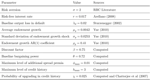
Table 5: Model parameters

Parameter Value Sources

Risk aversion = 2 RBC Literature

Risk-free interest rate r = 0:017 Arellano (2008)

Baseline output loss in default d= 0:02 Sturzenegger (2002)

Average endowment growth _g = 0:0042 Yue (2010)

Standard deviation of endowment growth shock g = 0:0253 Yue (2010)

Endowment growth AR(1) coe¢cient _g = 0:41 Yue (2010)

Discount factor = 0:75 Computed

Baseline bargaining power = 0:72 Computed

Maximum level of additional spread premia _max= 0:01 Computed

Maximum level of credit history hmax= 3 Computed

Probability of upgrading in credit history = 0:025 Computed and Chatterjee et al (2007)

6.2 Numerical results on equilibrium properties

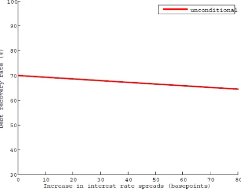
In this subsection, we cover the equilibrium properties of the model. Figure 4 shows the relationship

between increase in interest spreads and recovery rates unconditional on income states.26 _{As in}

Section 3, we de…ne increase in spreads as the di¤erence between spreads with defaults and those

with non-defaults. We calculate spreads after default based on both expected recovery rates for

next default and agreed additional spread premia, and spreads with non-defaults are measured with

expected recovery rates for the current default. It is clear that there is a negative relationship between

recovery rates and increase in interest spreads. If the increase in spreads is high, recovery rate is low

and vice versa. One interpretation is that if the country repays a large fraction of its debt at the

renegotiations, long-term borrowing costs will be small. In the case of Yue (2010), the slope of the

contract curve is vertical as shown in Appendix C. A driving force which makes our results di¤erent

from Yue (2010) is additional spread premia agreed at the debt restructurings.

2 6_{Figure A2 in Appendix D displays the relationship between increase in interest spreads and recovery rates conditional}

Figure 4: Relationship between increase in interest spreads and recovery rates

Figure 5: Default probability under baseline case

Figure 5 illustrates the baseline default probability at the mean income level. It is apparent that

the default probability is weakly increasing with the credit history. At the higher level of credit

history, additional increase in spreads on the newly issued bonds, determined at the previous debt

renegotiation, leads to higher costs for the country to borrow from investors compared with credit

history ht= 0.

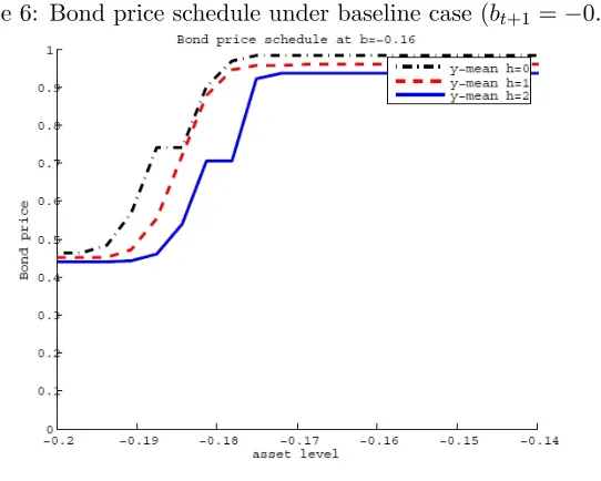
Figure 6 presents that bond price is also weakly decreasing with respect to the credit history.

What play behind are additional spread premia agreed at the past debt renegotiations: as explained

in detail in Section 6.4, these additional spread premia decrease the bond price both directly and

Figure 6: Bond price schedule under baseline case (bt+1 = 0:16)

6.3 Simulation results

We conduct 1000 rounds of simulations with 2000 periods per round and then extract 80 observations

before and 25 observations after each default event in stationary distribution to compute statistics.27

Bond spreads are from the J.P. Morgan’s Emerging Markets Bond Index Global (EMBIG) for

Ar-gentina for 1997Q1–2001Q4 and 2005Q3–2011Q3. Output data are seasonally adjusted from the

MECON for 1980Q1–2001Q4 and 2005Q3–2011Q3. Consumption and trade balance data are also

seasonally adjusted from the MECON for 1993Q1–2001Q4 and 2005Q3–2011Q3. Trade balance is

calculated as ratio to real GDP. Argetina’s external debt data are from the IMF WEO for 1980–2001

and 2005–2011. We compute two measures of the sovereign’s indebtness: the …rst measure is the

average external debt/GDP ratio. We also compute the ratio of the country’s debt service (including

short-term debt) to its GDP for Argentina. One advantage of our model compared with Yue (2010)

or Aguiar and Gopinath (2006) is that we obtain the statistics for post-default periods.

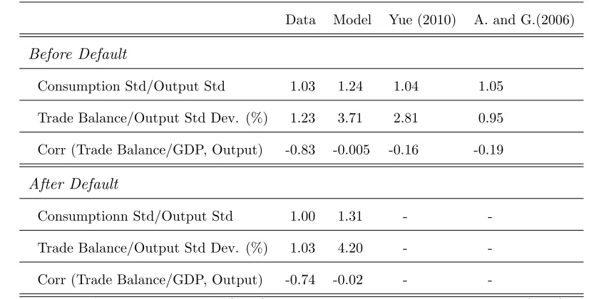
As apparent from Table 6, the model matches the business cycle statistics in data. For pre-default

periods, our model replicates volatile consumption and trade balance/GDP volatility, both of which

are prominent features of emerging economies business cycle models In addition, it also generates the

negative correlation between trade balance and output. However, a novelty of our model comes from

the better match of statistics with data in post-default periods, particilarly on consumption volatility

2 7_{We choose 80 observations prior to and 25 observations after a default event to compute the sample in the data}

and correlation of trade balance and output.

Table 6: Business Cycle Statistics

Data Model Yue (2010) A. and G.(2006)

Before Default

Consumption Std/Output Std 1.03 1.24 1.04 1.05

Trade Balance/Output Std Dev. (%) 1.23 3.71 2.81 0.95

Corr (Trade Balance/GDP, Output) -0.83 -0.005 -0.16 -0.19

After Default

Consumptionn Std/Output Std 1.00 1.31 -

-Trade Balance/Output Std Dev. (%) 1.03 4.20 -

-Corr (Trade Balance/GDP, Output) -0.74 -0.02 -

-Source: Aguiar and Gopinath (2006), Datastream, IMF WEO, MECON, Yue (2010)

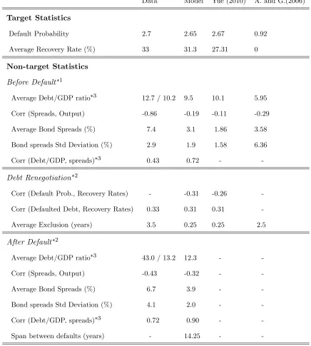
We move on to non-business cycle statistics of the model and data. First of all, in pre-default

periods, the model creates a moderate level of debt relative to data statistics. In the data, the total

debt service/GDP ratio is 10.2%. The model generates the average debt/GDP ratio of 10.4%. In

addition, the model also shows the relation among bond spreads, debt/GDP ratio and outputs as in

the data. Bonds spreads are possitively correlated with debt/GDP, but negatively correlated with

output. This is because default probability is high and recovery rates are low in low income states

resulting in high spreads. The average bond spreads is 3.1% in our simulations, lower than 7.4%

reported in the data, but higher than in Yue (2010). The volatility of bond spreads is 1.9% in our

simulation, close to the data (2.9%). The debt recovery rates are negatively correlated with default

probability.

What makes our model more distinctive is the model accounts the regularities in the post-default

periods. The average debt/GDP ratio is 12.3%, close to the debt service/GDP ratio of 13.2%. It is

clear that the model explains one prominent feature of average debt/GDP ratio in both pre-default

and post-default periods: the average debt/GDP ratio is higher in post-default period (12.3%) than

in pre-default period (10.4%). What is driving behind is increase in borrowing costs which forces

the sovereign to accumulate higher debts. Furthermore, our model provides the better match of the

periods. Even in the same low income states, the sovereign tends to accumulate higher debts in

post-default periods leading to higher spreads than in pre-post-default periods. This is also justi…ed by the

average bond spreads in post-default periods (3.9%) higher than one in pre-default periods (3.0%). It

also shows an obvious improvement of the average spreads compared with Yue (2010). On contrary,

the volatility of bond sreads in the post-default periods remains the same as in pre-crisis period.

Table 7: Model statistics for Argentina

Data Model Yue (2010) A. and G.(2006)

Target Statistics

Default Probability 2.7 2.65 2.67 0.92

Average Recovery Rate (%) 33 31.3 27.31 0

Non-target Statistics

Before Default 1

Average Debt/GDP ratio 3 12.7 / 10.2 9.5 10.1 5.95

Corr (Spreads, Output) -0.86 -0.19 -0.11 -0.29

Average Bond Spreads (%) 7.4 3.1 1.86 3.58

Bond spreads Std Deviation (%) 2.9 1.9 1.58 6.36

Corr (Debt/GDP, spreads) 3 0.43 0.72 -

-Debt Renegotiation 2

Corr (Default Prob., Recovery Rates) - -0.31 -0.26

-Corr (Defaulted Debt, Recovery Rates) 0.33 0.31 0.31

-Average Exclusion (years) 3.5 0.25 0.25 2.5

After Default 2

Average Debt/GDP ratio 3 43.0 / 13.2 12.3 -

-Corr (Spreads, Output) -0.43 -0.32 -

-Average Bond Spreads (%) 6.7 3.9 -

-Bond spreads Std Deviation (%) 4.1 2.0 -

-Corr (Debt/GDP, spreads) 3 0.72 0.90 -

-Source: Aguiar and Gopinath (2006), Datastream, IMF WEO, MECON, Yue (2010)

1_{: Data statistics before default correspond to sample of 1980Q1-2001Q4 (output), 1990Q1-2001Q4 (trade}

balance and consumption), and 1997Q1-2001Q4 (spreads). 2: Data statistics during and after debt

renegotiation correspond to samples of 2002Q1-2005Q2 and of 2005Q3-2011Q3 respectively. 3: Two

measures are the average total debt service (interest and amortization paid) and the average short-term debt

outstanding at year end. We use the second measure (short-tern debt outstanding) to calculate correlation.

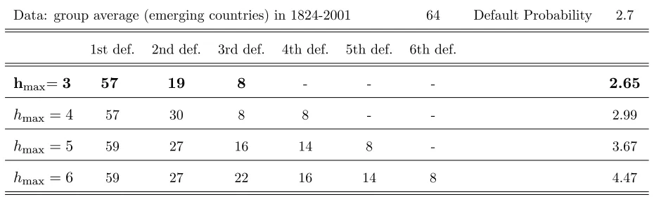
Furthermore, we calculate the average time spans between defaults based on 2000 rounds of

simulations by extracting the initial 200 periods of total 2000 periods per round. Table 8 reports that

the average spans between defaults are weakly decreasing with respect to the number of past debt

renegotiations. This feature is robust to extensions related with the upper limits of credit history.

Table 8: Average time spans between defaults (quarters)

Data: group average (emerging countries) in 1824-2001 64 Default Probability 2.7

1st def. 2nd def. 3rd def. 4th def. 5th def. 6th def.

h_max=3 _{57 19 8 - - - 2.65}

hmax= 4 57 30 8 8 - - 2.99

hmax= 5 59 27 16 14 8 - 3.67

hmax= 6 59 27 22 16 14 8 4.47

6.4 Impacts of additional spread premia

In this subsection, we explain how additional spread premia agreed at past debt renegotiations lead

to increase in spreads, which distinguishes this paper with the previous work. Based on equation (19)

and (20), we can rewrite interest spreads for credit history ht 1 as follows.

s(bt+1; ht; yt) =

0 if bt+1 0 1+r+ (bt;ht;yt)

[1 p(bt+1;ht;yt)+p(bt+1;ht;yt) (bt+1;ht;yt)] (1 +r) otherwise

(20a)

Given risk-free rate (r), total spreads can be decomposed into two factors:

(A) spread components based on "pure" default probability,

(B) spread components based on impact of additional spread premia.

irrelevant to the credit history. It is the measure of interest spreads used in Yue (2010). The latter

is how much the term (bt; ht; yt), increases total spreads. It can be regarded as spread components

associated with the past default history.

Figure 7 displays both the total spreads and spread components measured with "pure" default

probability. The spread components measured with "pure" default probability is equal to (A). The

total spreads is de…ned by equation (20a). The di¤erence between these two corresponds to (B),

which can be interpreted as spread components associated with the past default history. It is clear

that total spreads deviate from spread components measured with "pure" default probability when

the debt-to-GDP ratio is above the threshold value 0.175 in the mean income state.

Figure 7: The total spreads and spreads based on "pure" default probability

6.5 A brief summary of quantitative analysis

Our major …ndings can be summarized as follows. First of all, by incorporating additional spread

premia, the model accommodates an observed pattern of lower recovery rates associated with larger

increases in yield spreads. Second, we show that default probability is weakly increasing with credit

history, given the same debt-to-GDP ratio. Third, simulation exercises show that our model accounts

both business cycle and non-business cycle regularities in the post-default periods, which di¤erentiates

this model from the previous work Finally, interest spreads in our model can be decomposed into two

parts: spread components based on "pure" default probability, and spread components associated

7

Model implications

In this section, we explore the determinants of the slope of the contract curve. Moreover, we consider

possible implications derived from the changes in length of creditors’ memory and size of additional

spread premia.

7.1 Determinants of the slope of the contract curve

We focus on factors which a¤ect the value of the slope of the contract curve. Table 9 shows the values

of the slope under di¤erent values for the discount factor, the maximum level of additional spread

premia, output cost, risk-free rate and probability of upgrading in credit history.28 _{The impacts of a}

change in one parameter, leaving all other parameters …xed are indicated respectively.

Table 9: Values of the slope of the contract curve under di¤erent parameter values

Data -0.62

Discount factor Slope Maximum level of additional spread premia Slope Output cost Slope

= 0:81 -0.03 _max= 0:025 -0.03 d= 0:025 -0.10

=0_:75 _{-0.07 max=}0_:01 _{-0.07 d=}0_:0225 _-0.08

max= 0:005 -0.12 d= 0:02 -0.07

Risk-free interest rate Probability of upgrading in credit history

r = 0:03 -0.08 = 0 -0.07

r₌0_:017 _{-0.07 =}0_:025 _-0.07

r = 0:01 -0.05 = 0:075 -0.07

Note: all the values are those at the default

First, the slope gets steeper as the discount factor decreases. From the country’s perspective, the

cost of paying to one additional unit of defaulted debt at the renegotiation relative to the cost of

facing one additional unit of increase in spreads, gets smaller as the discount factor decreases. Next,

when the maximum level of additional spread premia is reduced to 50 basis points ( _max = 0:005),

the absolute value of the slope increases. Since increase in spreads is limited to a lower level due to

the lower maximum level of additional spread premia, paying one additional unit of defaulted debt at

2 8_{Changes in value for bargaining power has an ambitious impact on the slope of the contract curve. Rather than the}

the renegotiation is less costly relative to paying one additional unit of spread increases in the future

period.

On contrary, an increase in output cost leads to an increase in the absolute value of the slope. As

the cost of default is larger for the country, relative cost of paying one additional unit of defaulted

debt at the renegotiation instead of facing one additional unit of increase in spreads decreases taking

into account the cost of next default.

The absolute value of slope increases as the risk-free rate increases. Total size of increase in

spreads gets larger associated with an increase in risk-free interest rate. Given the constant change in

recovery rate, it makes the slope of the contract curve more ‡atter, indicating that from the country’s

point of view, paying one additional unit of defaulted debt at the renegotiation is less costly than

paying one additional unit of spread returns in the future periods. Lastly, probability of upgrading

in credit history does not a¤ect the value of slope.

7.2 Duration and size of additional spread premia

Determination of both recovery rates and additional spread premia at the debt renegotiation plays

an important role in our model. Probability of upgrading in credit history and maximum level of

additional spread premia are two key parameters which specify the duration and size of deterioration

in long-term credit. Table 10 reports how changes in these parameter values in‡uence the non-business

cycle statistics.29

Increase in probability of upgrading reduces the average debt/GDP ratio, average bond spreads

and correlation between debt/GDP and spreads. As the probability of upgrading in credit history

gets higher, length of deterioration in long-run credit gets shorter. The sovereign tends to have lower

levels of debt and spreads, which also lead to lower correlation between debt/GDP ratio and spreads.

On the contrary, not only the average debt/GDP, average bond spreads and correlation between

debt/GDP and spreads, but also the default probability increases as the upper limit of additional

spread premia gets higher. The maximum level of additional spread premia identi…es the size of

deterioration in long-term credit, given the …xed duration. Associated with increase in borrowing

costs, the sovereign accumulates more debts leading to increases in both spreads and probability in

2 9_{Changes in parameter values of both probability in credit history and maximum level of additional spread premia}

default.

Table 10: Statistics for di¤erent levels of upgrading in credit history and additional spread premia

Probability of upgrading Maximum level of additional spread premia

= 0 =0_:025 _{= 0:075 max= 0:005 max=}0_:01 _{max= 0:025}

Default Probability 2.67 2.65 2.65 2.55 2.65 3.04

Average Recovery Rate (%) 31.9 31.3 31.9 32.2 31.3 31.5

Before Default 1

Average Debt/GDP ratio 3 10.4 9.5 10.4 10.4 9.5 11.8

Corr (Spreads, Output) -0.08 -0.06 -0.08 -0.05 -0.06 -0.13

Average Bond Spreads (%) 3.4 3.0 3.4 3.2 3.0 4.0

Bond spreads Std Deviation (%) 1.9 1.9 1.9 1.8 1.9 2.4

Corr (Debt/GDP, spreads) 3 0.82 0.72 0.82 0.81 0.72 0.82

After Default 2

Average Debt/GDP ratio 3 10.9 12.3 10.9 10.9 12.3 12.4

Corr (Spreads, Output) -0.25 -0.41 -0.27 -0.29 -0.41 -0.21

Average Bond Spreads (%) 3.9 3.9 3.9 3.6 3.9 4.6

Bond spreads Std Deviation (%) 2.0 2.0 2.0 1.9 2.0 2.6

Corr (Debt/GDP, spreads) 3 0.90 0.90 0.90 0.88 0.90 0.89

8

Conclusion

Emerging countries that have defaulted on their debt repayment obligations in the past are more

likely to default again in the future than are non-defaulters with the same debt-to-GDP ratio. This

paper explains this stylized fact within a dynamic stochastic general equilibrium framework that

explicitly models debt renegotiations between a defaulting country and its creditors. Speci…cally, the

model extends the existing literature by allowing defaulters and creditors to bargain not just over

recovery rates, but also over the rate of return o¤ered on newly-issued debt. Quantitative analysis of

the model reveals that the equilibrium probability of default for a given debt-to-GDP level is weakly