Technical Appendix to "Macroeconomic effects of public sector unions"

(1)

Munich Personal RePEc Archive

Technical Appendix to "Macroeconomic

effects of public sector unions"

Vasilev, Aleksandar

AUBG

June 2013

Online at

https://mpra.ub.uni-muenchen.de/68235/

(2)

Technical Appendix to ”Macroeconomic effects of public

sector unions

Aleksandar Vasilev

∗

December 6, 2015

1 Technical Appendix

1.1 Optimality conditions

1.1.1 Firm’s problem

The profit function is maximized when the derivatives of that function are set to zero.

Therefore, the optimal amount of capital - holding the level of technologyAt and labor input

Ntp constant - is determined by setting the derivative of the profit function with respect to

K_tp equal to zero. This derivative is

(1−_θ₎_A_t₍_Kp t)

−_θ

(N_tp)θ₍_Kg

t)ν−rt = 0 (1)

where (1−_θ₎_A_t(_K_tp₎−θ

(Ntp)θ(Ktg)ν is the marginal product of capital because it expresses

how much output will increase if capital increases by one unit. The economic interpretation

of this First-Order Condition (FOC) is that in equilibrium, firms will rent capital up to

the point where the benefit of renting an additional unit of capital, which is the marginal

product of capital, equals the rental cost, i.e the interest rate.

rt = (1−θ)At(Ktp)

−θ

(N_tp)θ(K_tg)ν (2)

∗_{Asst. Professor, American University in Bulgaria, Department of Economics, Blagoevgrad 2700,}

(3)

Now, multiply byK_tp and rearrange terms. This gives the following relationship:

K_tp(1−_θ₎_A_t(_Kp t)

−θ

(N_tp)θ(K_tg)ν =rtKtp or (1−θ)Yt =rtKtp (3)

because

Ktp(1−θ)At(Ktp)

−θ

(Ntp)θ(Ktg)ν =At(Ktp)1

−θ

(Ntp)θ(Ktg)ν = (1−θ)Yt

To derive firms’ optimal labor demand, set the derivative of the profit function with respect

to the labor input equal to zero, holding technology and capital constant:

θAt(Ktp)1

−θ

(Ntp)θ

−1

(Ktg)ν −wpt = 0 or wpt =θAt(Ktp)1

−θ

(Ntp)θ

−1

(Ktg)ν (4)

In equilibrium, firms will hire labor up to the point where the benefit of hiring an additional

hour of labor services, which is the marginal product of labor, equals the cost, i.e the hourly

wage rate.

Now multiply both sides of the equation by N_tp and rearrange terms to yield

NtpθAt(Ktp)1

−θ

(Ntp)θ

−1

(Ktg)ν =wtpNtp or θYt =wptNtp (5)

Next, it will be shown that in equilibrium, economic profits are zero. Using the results above

one can obtain

Πt = Yt−rtKtp−wptNtp =Yt−(1−θ)Yt−θYt= 0 (6)

Indeed, in equilibrium, economic profits are zero.

1.1.2 Consumer problem

Set up the Lagrangian

L₍_C_t_{, K}p t+1, N

p

t; Λt) =E0 ∞

X

t=0

(

(Ct+ωGct)ψ(1−Nt)(1

−ψ)

1−α

−₁

1−_α + (7)

+Λt

"

(1−_τl₎₍_w_tp_N_tp₊_w_tg_N_tg_{) + (1}−_τk₎_r_t_K_tp ₊

+τkδpKtp−(1 +τc)Ct−Ktp+1+ (1−δ)K

p t

(4)

This is a concave programming problem, so the FOCs, together with the additional,

bound-ary (”transversality”) conditions for private physical capital and government bonds are both

necessary and sufficient for an optimum.

To derive the FOCs, first take the derivative of the Lagrangian w.r.t Ct (holding all other

variables unchanged) and set it to 0,i.e. L_C

t = 0. That will result in the following expression

βt

(

1−_α 1−_α

(Ct+ωGct)ψ(1−Nth)(1

−_ψ₎

−_α

×

ψ(Ct+ωGct)ψ

−1

(1−_Nh t)(1

−ψ)

−_{Λt(1 +}_τc₎

)

= 0 (8)

Cancel the βt _{and the 1}₋_α _{terms to obtain}

−ψ)

−_α

ψ(Ct+ωGct)ψ

−1

(1−_N_t₎(1−ψ)

−_Λ_t_{(1 +}_τc_{) = 0} ₍₉₎

Move Λt to the right so that

−ψ)

−α

ψ(Ct+ωGct)ψ

−1

(1−_N_t)(1−ψ)

= Λt(1 +τc) (10)

This optimality condition equates marginal utility of consumption to the marginal utility of

wealth.

Now take the derivative of the Lagrangian w.r.tK_tp₊₁ (holding all other variables unchanged)

and set it to 0, i.e. _L

Ktp+1 = 0. That will result in the following expression

βt

(

−_Λt₊_E_tΛt₊₁

(1−_τk₎_r_t₊₁₊_τk_δp _{+ (1}−_δp₎

)

= 0 (11)

Cancel the βt _{term to obtain}

−_Λt₊_βE_tΛt₊₁

(1−_τk₎_r_t₊₁₊_τk_δp_{+ (1}−_δp₎

= 0 (12)

Move Λt to the right so that

βEtΛt+1

(1−_τk₎_r_t₊₁₊_τk_δp_{+ (1}−_δp₎

(5)

Using the expression for the real interest rate shifted one period forward one can obtain

rt+1 = (1−θ)

Yt+1

K_tp₊₁

βEtΛt+1

(1−_τk₎₍₁−_θ₎Yt+1

K_tp₊₁ +τ

k_δp_{+ (1}₋_δp₎

= Λt (14)

This is the Euler equation, which determines how consumption is allocated across periods.

Take now the derivative of the Lagrangian w.r.t N_tp (holding all other variables unchanged)

and set it to 0, i.e. L_Np

t = 0. That will result in the following expression

βt

(

1−_α 1−_α

−ψ)

−α

×

(1−_ψ₎₍_C_t₊_ωGc

t)ψ(1−Nt)

−ψ

(−_{1) + Λ}_t₍₁−_τl₎_wp t

)

= 0 (15)

Cancel the βt _{and the 1}₋_α _{terms to obtain}

−ψ)

−α

(1−_ψ₎

Ct+ωGct 1−_N_t

ψ

(−_{1) + Λt(1}−_τl₎_wp

t = 0 (16)

Rearranging, one can obtain

−ψ)

−α

(1−_ψ₎₍_C_t₊_ωGc

t)ψ(1−Nt)

−ψ

= Λt(1−_τl₎_wp

t (17)

Plug in the expression for wh

t, that is,

wpt =θ

Yt

N_tp (18)

into the equation above. Rearranging, one can obtain

−_ψ₎

−α

(1−_ψ₎₍_C_t₊_ωGc

t)ψ(1−Nt)

−_ψ

= Λt(1−_τl₎_θ Yt

Ntp

(19)

Transversality conditions need to be imposed to prevent Ponzi schemes, i.e borrowing bigger

and bigger amounts every subsequent period and never paying it off.

lim t→∞β

t_Λ

(6)

1.1.3 The Objective Function of a Public Sector Union: Derivation

This subsection shows that the objective function in the government sector is a generalized

version of Stone-Geary monopoly union utility function used in Dertouzos and Pencavel

(1981) and Brown and Ashenfelter (1986). The utility function is

V(wg, Ng) = (wg −_w_¯g₎φ₍_Ng−_N¯g₎(1−φ)

, (21)

where φ and 1−_φ _{are the weights attached to public wage and hours, respectively, and ¯}_wg

and ¯Ng _{denote subsistence wage rate and hours. Since there is no minimum wage in the}

model, ¯wg _{= 0. Additionally, as public hours are assumed to be unproductive, it follows}

that ¯Ng _{= 0 as well. Therefore, the utility function simplifies to}

V(wg, Ng) = (wg)φ(Ng)(1−φ)

. (22)

Doiron (1992) uses a generalized representation, which encompasses (2) as a special case

when ρ→_0.

φ(Ng)−ρ

+ (1−_φ₎₍_wg−_w_¯₎−ρ

−1/ρ

, (23)

when ¯w= 0, the function simplifies to

φ(Ng)−ρ

+ (1−_φ₎₍_wg₎−ρ

−1/ρ

, (24)

Union objective function used in the paper is very similar to Doiron’s (1992) simplified

version:

(Ng)ρ+η(wg)ρ

1/ρ

, (25)

can be transformed to

(Ng)ρ+ φ (1−_φ₎(w

g₎ρ

1/ρ

, (26)

Collecting terms under common denominator

(1−_φ₎ (1−_φ₎(N

g₎ρ₊ φ (1−_φ₎(w

g₎ρ

1/ρ

(7)

Factoring out the common term

1 1−_φ

1/ρ

(1−_φ₎₍_Ng₎ρ₊_φ₍_wg₎ρ

1/ρ

, (28)

Note that the constant term

1 1−φ

1/ρ

>0 can be ignored, as utility functions are invariant

to positive affine transformations. After rearranging terms, the equivalent function

˜

V =

φ(wg)ρ+ (1−_φ₎₍_Ng₎ρ

1/ρ

. (29)

Take natural logarithms from both sides to obtain

ln ˜V = 1

ρln

φ(wg)ρ+ (1−_φ₎₍_Ng₎ρ

. (30)

Take the limit ρ→₀

lim

ρ→0ln ˜V = limρ→0

ln

φ(wg₎ρ_{+ (1}₋_φ₎₍_Ng₎ρ

ρ (31)

Apply L’Hopital’s Rule on the R.H.S. to obtain

lim

ρ→0ln ˜V = limρ→0

∂ ∂ρln

φ(wg₎ρ_{+ (1}₋_φ₎₍_Ng₎ρ

∂ρ ∂ρ

(32)

Thus

ln ˜V = lim ρ→0

φ(wgt)ρlnwg+ (1−φ)(Ng)ρlnNg

/

φ(wg₎ρ_{+ (1}₋_φ₎₍_Ng₎ρ

1 (33)

Simplify to obtain

ln ˜V =

limρ→0

φ(wg_t)ρ_ln_wg_{+ (1}₋_φ₎₍_Ng₎ρ_ln_Ng

limρ→0

φ(wg₎ρ_{+ (1}₋_φ₎₍_Ng₎ρ

=

φlnwg _{+ (1}₋_φ_{) ln}_Ng

φ+ (1−_φ₎ (34)

Therefore,

(8)

Exponentiate both sides of the equation to obtain

eln ˜V =eφlnwg+(1−φ) lnNg

. (36)

Thus

˜

V =eln(wg)φ+ln(Ng)(1−φ)

. (37)

or

˜

V =eln(wg)φ(Ng)(1−φ)

. (38)

Finally,

˜

V = (wg)φ(Ng)(1−φ)

(39)

Furthermore, government period budget constraint serves the role of a labor demand

func-tion. Additionally, the public sector demand curve will be subject to shock, resulting from

innovations to the fiscal shares. The balanced budget assumption is thus important in the

model setup. Since wage bill is a residual, if wage rate is increased, then hours need to be

decreased. Additionally, government period budget constraint can be expressed in the form

Ng ₌_Ng₍_wg_{) as}

Ng = τ

l_wp_Np ₊_τk₍_r₋_δp₎_Kp₊_τc_C₋_Gc₋_Gi₋_Gt

(1−_τl₎_wg (40)

Therefore, the problem in the government sector is reshaped in the standard formulation in

the union literature:

max wg_,NgV(w

g_{, N}g₎ _s.t. _Ng ₌_Ng₍_wg₎ ₍₄₁₎

Since union optimizes over both the public wage and hours, the outcome is efficient. The

solution pair is on the contract curve (obtained from FOCs), at the intersection point with

(9)

1.1.4 Public sector union optimization problem

The union solves the following problem:

max wtg,N

g t

(Ntg)ρ+η(wgt)ρ

1/ρ

(42)

s.t

Gc_t+Gt_t+Gi_t+wtgNtg =τcCt+τkrtKtp−τkδpKt+τl[wptNtp +wgtNtg] (43)

Setup the Lagrangian

V₍_wg

t, Ntg;νt) = max wgt,N

g t

(Ntg)ρ+η(wgt)ρ

1/ρ

(44)

−_ν_t

Gc_t +Gt_t+Gi_t+wtgNtg−τcCt−τkrtKtp+τkδpKt−τl[wtpNtp+wtgNtg]

Optimal public employment is obtained, when the derivative of the government Lagrangian

is et to zero, i.e V

Ntg = 0

(1/ρ)

(N_tg)ρ₊_η₍_wg t)ρ

(1/ρ)−1

ρ(N_tg)ρ−₁

−₍₁−_τl₎_ν_t_wg

t = 0 (45)

or, when ρ is canceled out and (1−_τl₎_ν_t_wg

t put to the right

(N_tg)ρ+η(wg_t)ρ

(1/ρ)−₁

(N_tg)ρ−1

= (1−_τl₎_ν_t_wg

t (46)

Optimal public wage is obtained, when the derivative of the government Lagrandean is et

to zero, i.e V_wg t = 0

(1/ρ)

(N_tg)ρ+η(w_tg)ρ

(1/ρ)−1

ηρ(wg_t)ρ−1

−₍₁−_τl₎_ν_t_Ng

t = 0 (47)

or, when ρ is canceled out and(1−_τl₎_ν

tNtg term put to the right

(N_tg)ρ+η(w_tg)ρ

(1/ρ)−1

η(w_tg)ρ−1

= (1−_τl₎_ν_t_Ng

t (48)

Divide (11.1.46) and (11.1.48) side by side to obtain

(Ntg)ρ+η(wgt)ρ

(1/ρ)−1

(Ntg)ρ

−₁

(Ntg)ρ+η(wtg)ρ

(1/ρ)−1

η(wtg)ρ−1

= (1−τ l₎_ν

twtg (1−_τl₎_ν

tNtg

(10)

Cancel out the common terms

(Ntg)ρ

−₁

η(w_tg)ρ−1 =

wtg

N_tg (50)

Now cross-multiply to obtain

(N_tg)ρ

η = (w

g

t)ρ (51)

Hence

wtg =

1

η

1/ρ

Ntg (52)

The wage bill expression, which is obtained after simple rearrangement of the government

budget constraint, is as follows

wtgNtg =

τc_C

t+τkrtKtp−τkδpKt+τlwptNtp−Gtc−Gtt−Git

1−_τl (53)

Use the wage bill equation and the relationship between public wage and employment in

order to obtain

wtg =η

−1

2ρ

τc_C

t+τkrtKtp−τkδpKt+τlwtpNtp−Gtc−Gtt−Git 1−_τl

1₂

(54)

and

N_tg =η21ρ

τc_C

t+τkrtKtp−τkδpKt+τlwptN p

t −Gct −Gtt−Git 1−_τl

1₂

(11)

1.2 Log-linearized model equations

1.2.1 Linearized market clearing

ct+kpt+1+gtc+gti−(1−δp)k p

t = yt (56)

Take logs from both sides to obtain

ln[ct+kpt+1+gtc+gti−(1−δp)k p

t] = ln(yt) (57)

Totally differentiate with respect to time

dln[ct+kpt+1+gtc+gti−(1−δp)k p t]

dt = dln(yt) (58)

[ 1

c+gc ₊_gi₊_δp_kp][

dct dt c c + dgc t dt g g + dgi t dt gi

gi +

dk_tp₊₁ dt

kp

kp −(1−δ p₎dk

p t

dt kp

kp] =

dyt

dt

1

y (59)

Define ˆz = dzt

dt

1

z. Thus passing to log-deviations 1

y[ˆctc+ ˆg

c

tgc + ˆgitgi + ˆk p

t+1kp−(1−δp)ˆk

p

tkp] = ˆyt (60)

ˆ

ctc+ ˆgtcgc + ˆgitgi + ˆk p

t+1kp−(1−δp)ˆk

p

tkp = yyˆt (61)

kpˆkp_t₊₁ = yyˆt−ccˆt−gcˆgtc−giˆgti+ (1−δp)kpkˆ p

t (62)

1.2.2 Linearized production function

yt = at(kpt)1

−θ

(np_t)θ(kg_t)ν (63)

Take natural logs from both sides to obtain

lnyt = lnat+ (1−θ) lnktp+θlnn p

t +νlnk g

t (64)

Totally differentiate with respect to time to obtain

dlnyt

dt =

dlnat

dt + (1−θ) dlnkp_t

dt +θ

dlnnp_t

dt +ν

dlnkg_t

dt (65) 1 y dyt dt = 1 a dat dt +

1−_θ

kp

dkp_t dt +

θ np

dnp_t

dt +

ν kg

dk_tg

dt (66)

Pass to log-deviations to obtain

0 = −_y_ˆ_t_{+ (1}−_θ_)ˆ_kp

t + ˆat+θnˆpt +νkˆ g

(12)

1.2.3 Linearized FOC consumption

[(ct+ωgtc)ψ(1−nt)(1

−ψ)

]−α

ψ(ct+ωgtc)ψ

−1

(1−_n_t)(1−ψ)

= (1 +τc)λt (68)

Simplify to obtain

ψ(ct+ωgtc)ψ

−1−αψ

(1−_n_t)(1−α)(1−ψ)

= (1 +τc)λt (69)

lnψ(ct+ωgtc)ψ

−₁−_αψ

(1−_n_t₎(1−_α₎₍₁−_ψ₎

= ln(1 +τc_{) + ln}_λ

t (70)

ln(ct+ωgtc)ψ

−₁−_αψ

(1−_n_t₎(1−_α₎₍₁−_ψ₎

= ln(1 +τc_{) + ln}_λ

t (71)

(ψ−₁−_αψ_{) ln(}_c_t₊_ωgc

t) + (1−α)(1−ψ) ln(1−nt) = ln(1 +τc) + lnλt (72)

(ψ−₁−_αψ₎dln(ct+ωg c t)

dt + (1−α)(1−ψ)

dln(1−_n_t)

dt =

= dln(1 +τ c₎

dt +

dlnλt

dt (73)

(ψ−₁−_αψ₎ 1

c+ωgc(

dct

dt +ω dgc

t

dt ) + (1−α)(1−ψ)

−₁ 1−_n

dnt dt = dλt dt 1 λ (74)

(ψ−₁−_αψ₎

c+ωgc

dct

dt c c +

ω(ψ−₁−_αψ₎

c+ωgc

dgc t

dt gc

gc +

−₍₁−_α₎₍₁−_ψ₎ 1 1−_n

dnt dt n n = dλt dt 1 λ (75)

c(ψ−₁−_αψ₎

c+ωgc cˆt+

ωgc₍_ψ₋₁₋_αψ₎

c+ωgc gˆ c

t −(1−α)(1−ψ)

n

1−_nnˆ = ˆλt (76) Since

ˆ

n = n

p

np₊_ngˆn

p₊ ng

np₊_ngnˆ g ₌ np

n nˆ

p₊ ng

nnˆ

g_, ₍₇₇₎

and consumers choose np _{only, pass to log-deviations to obtain}

c+ωgc cˆt+

cc₊_ωg gˆ c

t −(1−α)(1−ψ)

n

1−_n

np

np ₊_ngˆn

p _{= ˆ}_λ

t (78)

Since n=np ₊_ng_{, it follows that}

c+ωgc ˆct+

c+ωgc ˆg c

t −(1−α)(1−ψ)

np 1−_nnˆ

(13)

1.2.4 Linearized no-arbitrage condition for capital

λt = βEtλt+1[(1−τk)rt+1+τkδp+ (1−δp)] (80)

Substitute out rt+1 on the right hand side of the equation to obtain

λt = βEt[λt+1((1−τk)(1−θ)

yt+1

k_tp₊₁ +τ

k_δp_{+ 1}₋_δp_)] ₍₈₁₎

Take natural logs from both sides of the equation to obtain

lnλt = lnEt[λt+1((1−τk)(1−θ)

yt+1

k_tp₊₁ +τ

k_δp_{+ 1}₋_δp_)] ₍₈₂₎

dlnλt

dt =

dlnEt[λt+1((1−τk)(1−θ)y_ktp+1 t+1 +τ

k_δp_{+ 1}₋_δp_)]

dt (83)

1

λ dλt

dt =Et

(

1

λ((1−_τk₎₍₁₋_θ₎y

kp + 1−δp+τkδp

×

"

((1−_τk₎₍₁−_θ₎y

kp +τ

k_δp _{+ 1}₋_δp₎dλt+1

dt λ λ

+λ(1−τ

k₎₍₁₋_θ₎

kp

dyt+1

dt y y −

λ(1−_τk₎₍₁−_θ₎_y (kp₎2

dk_tp₊₁ dt

kp

#)

(84)

ˆ

λt=Et

(

ˆ

λt+1+

(1−_τk₎₍₁−_θ₎_y ((1−_τk₎₍₁₋_θ₎yt+1

kpt+1 +τ

k_δp_{+ 1}₋_δp₎_kpyˆt+1

− (1−τ

k₎₍₁₋_θ₎_y

((1−_θ₎yt+1

ktp+1 +τ

k_δp_{+ 1}₋_δp₎_kpkˆ p t+1

)

(85)

Observe that

(1−_τk₎₍₁−_θ₎yt+1

k_tp₊₁ +τ

k_δp_{+ 1}₋_δp _{= 1}_/β ₍₈₆₎

Plug it into the equation to obtain

ˆ

λt = Et

ˆ

λt+1+

β(1−_τk₎₍₁−_θ₎_y

kp yˆt+1−

β(1−_τk₎₍₁−_θ₎_y

kp ˆk

p t+1

(87)

ˆ

λt = Etλˆt+1+

β(1−_τk₎₍₁−_θ₎_y

kp Etˆyt+1−

β(1−_τk₎₍₁−_θ₎_y

kp Etˆk

p

(14)

1.2.5 Linearized MRS

(1−_ψ₎₍_c_t₊_ωgc

t) = ψ(1−nt)

(1−_τl₎ (1 +τc₎θ

yt

npt

(89)

ln(1−_ψ₎₍_c_t₊_ωgc

t) = lnψ(1−nt)

(1−_τl₎ (1 +τc₎θ

yt

npt

(90)

ln(ct+ωgct) = ln(1−nt) + lnyt−lnnpt (91)

dln(ct+ωgtc)

dt =

dln(1−_n_t)

dt +

dlnyt

dt −

dlnnpt

dt (92)

1

c+ωgc(

dct

dt +ω dgc

t

dt ) = −

1 1−_n

dnt dt + 1 y dyt dt − 1 np

dnp_t

dt (93)

1

c+ωgc

dct

dt c c+

ω c+ωgc

dgc t

dt gc

gc = −

1 1−_n

dnt dt n n + 1 y dyt dt − 1 np

dnpt

dt (94)

c c+ωgc

dct

dt

1

c + ωgc

c+ωgc

dgc t

dt

1

gc = −

n

1−_n

dnt dt 1 n + 1 y dyt dt − 1 np

dnp_t

dt (95)

c

c+ωgccˆt+

ωgc

c+ωggˆ

c

t = −

n

1−_nnˆ+ ˆyt−nˆ p

t (96)

Since

ˆ

n= n

p

np₊_ngnˆ

p₊ ng

np₊_ngnˆ

g_, ₍₉₇₎

and noting that consumers are only choosing np_{, then}

c

c+ωgccˆt+

ωgc

c+ωgcˆg c

t = −

n

1−_n

np

np₊_ngˆn p_{+ ˆ}_y

t−nˆpt (98)

c

c+ωgccˆt+

ωgc

c+ωgcˆg c

t = −

n

1−_n

np

np₊_ngˆn p_{+ ˆ}_y

t−nˆpt (99)

c

c+ωgcˆct+

ωgc

c+ωgcgˆ c

t = −

1 + n 1−_n

np

np₊_ng

ˆ

np+ ˆyt (100)

Since n=np ₊_ng_{, it follows that}

c

c+ωgcˆct+

ωgc

c+ωgcgˆ c

t = −

1 + n p 1−_n

ˆ

np+ ˆyt (101)

c

c+ωgcˆct+

ωgc

c+ωgcˆg c t +

1 + n p 1−_n

ˆ

(15)

1.2.6 Linearized private capital accumulation

k_tp₊₁ = it+ (1−δp)ktp (103)

lnkp_t₊₁ = ln(it+ (1−δp)ktp) (104)

dlnkp_t₊₁

dt =

1

i+ (1−_δp₎_kp

d(it+ (1−δp)ktp)

dt (105)

Observe that since

i=δpkp, it follows that i+ (1−_δp₎_kp ₌_δp_kp_{+ (1}₋_δp₎_kp ₌_kp_. _Then ₍₁₀₆₎

dk_tp₊₁ dt

1

kp =

1

kp

dit

dt i i +

kp

i+ (1−_δp₎_kp t

dkp_t dt

kp

kp (107)

ˆ

kp_t₊₁ = δ p_kp

kp ˆit+

(1−_δp₎_kp

kp kˆ p

t (108)

ˆ

k_tp₊₁ = δpˆit+ (1−δp)ˆktp (109)

1.2.7 Linearized government capital accumulation

kg_t₊₁ = g_ti+ (1−_δg₎_kg

t (110)

lnk_tg₊₁ = ln(g_ti+ (1−_δg₎_kg

t) (111)

dlnk_tg₊₁

dt =

1

gi_{+ (1}₋_δg₎_kg

d(git+ (1−δg)ktg)

dt (112)

Observe that since

(16)

it follows that

gi+ (1−_δg₎_kg ₌_δg_kg_{+ (1}−_δg₎_kg ₌_kg_. ₍₁₁₄₎

Hence,

dk_tg₊₁ dt

1

kg = 1 kg dgi t dt gi

gi +

kg

x+ (1−_δg₎

dkg_t dt

kg

kg (115)

ˆ

k_tg₊₁ = δ g_kg

kg ˆg i t+

(1−_δg₎_kg

kg ˆk g

t (116)

Cancel out the kg _{terms to obtain}

ˆ

k_tg₊₁ = δgˆg_ti+ (1−_δg_)ˆ_kg

t (117)

1.2.8 Public wage rate rule

wg_t =η−1

2ρ

τc_c

t+τkrtktp−τkδpk p t +τlw

p tn

p

t −gct−gtt−gti 1−_τl

1₂

(118)

lnwgt =− 1

2ρlnη−

1

2ln(1−τ l_{) +}

1 2ln

τcct+τkrtktp−τkδpktp+τlwtpnpt −gct −gtt−gti

(119)

dlnwgt

dt = 1 2 d dtln

τcct+τkrtktp−τkδpk p t +τlw

p tn

p

t −gct −gtt−gti

(120)

Observe that

τkrtkpt −τkδpkt+τlwtpnpt =τk(1−θ)yt+τlθyt−τkδpkpt =

=

τk(1−_θ_{) +}_τl_θ

yt−τkδpktp (121)

Also

(1−_τl₎_wg_ng ₌_τc_c_{+ [}_τk₍₁−_θ_{) +}_τl_θ_]_y−_τk_δp_kp−_gc−_gi−_gt

(17)

Thus

dw_tg dt

1

wg = 1 2

1 (1−_τl₎_wg_ng

τcdct dt + [τ

k₍₁₋_θ_{) +}_τl_θ_]dyt

dt −τ

k_δpdk p t dt − dgc t dt − dgi t dt − dgt t dt (123)

dw_tg dt

1

wg = 1 2

1

(1−_τl₎_wg_ng ×

τcdct dt

c c+

τk(1−_θ_{) +}_τl_θ

dyt

dt y y −τ

k_δpdk p t

dt kp

kp −

dgc t

dt gc

gc −

dgi t

dt gi

gi −

dgt t dt gt gt (124)

dw_tg dt

1

wg =

(1/2)τc_c (1−_τl₎_wg_ng

dct

dt

1

c +

(1/2)

τk₍₁₋_θ_{) +}_τl_θ

y

(1−_τl₎_wg_ng

dyt

dt

1

y

−(1/2)τ k_δp_kp (1−_τl₎_wg_ng

dktp

dt

1

kp −

(1/2)gc (1−_τl₎_wg_ng

dgc t

dt

1

gc

− (1/2)g i

(1−_τl₎_wg_ng

dgi t

dt

1

gi −

(1/2)gt (1−_τl₎_wg_ng

dgt t

dt

1

gt (125)

ˆ

wgt =

(1/2)τc_c (1−_τl₎_wg_ngcˆt+

(1/2)

τk₍₁₋_θ_{) +}_τl_θ

y

(1−_τl₎_wg_ng yˆt

−(1/2)τ k_δp_kp

(1−_τl₎_wg_ngˆkt−

(1/2)gc (1−_τl₎_wg_nggˆ

c t −

(1/2)gi (1−_τl₎_wg_ngˆg

i t−

(1/2)gt (1−_τl₎_wg_nggˆ

t

t (126)

1.2.9 Public hours/employment rule

ng_t = η1ρwg

t (127)

lnngt = 1

ρlnη+ lnw

g

t (128)

Totally differentiate both sides to obtain

dlnng_t

dt =

dlnwg_t

dt (129)

dngt

dt

1

ng =

dwgt

dt

1

wg (130)

ˆ

(18)

1.2.10 Total hours/employment

nt = ngt +n p

t (132)

lnnt = ln(ngt +n p

t) (133)

Totally differentiate to obtain

dlnnt

dt =

dln(ng_t +np_t)

dt (134) dnt dt 1 n =

dngt

dt +

dnpt

dt 1 n (135) dnt dt 1 n =

dngt

dt ng

ng +

dnpt

dt np np 1 n (136) dnt dt 1 n =

dng_t dt

1

ng

n +

dnp_t dt

1

np

n (137)

ˆ

nt =

ng

n nˆ

g t +

np

n nˆ

p

t (138)

1.2.11 Linearized private wage rate

wpt =θ

yt

np_t (139)

lnwtp = lnθ+ lnyt−lnnpt (140)

dlnwp_t

dt =

dlnθ

dt +

dlnyt

dt −

dlnnp_t

dt (141)

Simplify to obtain

dwp_t dt

1

wp =

dyt

dt

1

y − dnp_t

dt

1

np (142)

ˆ

(19)

1.2.12 Linearized real interest rate

rt=θ

yt

kpt

(144)

lnrt = lnθ+ lnyt−lnktp (145)

dlnrt

dt =

dlnθ

dt +

dlnyt

dt −

dlnk_tp

dt (146)

Simplify to obtain

dr dt

1

r = dyt

dt

1

y − dktp

dt

1

kp (147)

ˆ

rt = ˆyt−ˆktp (148)

1.2.13 Public/private wage ratio

rwt = wgt/wpt (149)

Take logs from both sides of the equation

lnrwt = lnwtg−lnw p

t (150)

dlnrwt

dt =

dlnwtg

dt −

dlnwpt

dt (151)

drwt

dt

1

rw =

dwg_t dt

1

wg −

dw_tp dt

1

wp (152)

ˆ

(20)

1.2.14 Public/private hours/employment ratio

rlt = ngt/n p

t (154)

Take logs from both sides of the equation

lnrlt = lnngt −lnnpt (155)

dlnrlt

dt =

dlnng_t

dt −

dlnnp_t

dt (156)

drlt

dt

1

rl =

dngt

dt

1

ng −

dnpt

dt

1

np (157)

ˆ

rlt = ˆngt −nˆ p

t (158)

1.2.15 Linearized technology shock process

lnat+1 = ρalnat+ǫat+1 (159)

dlnat+1

dt = ρa

dlnat

dt +

dǫa t+1

dt (160)

dat+1

dt = ρa

dat

dt +ǫ

a

t+1 (161)

where for t = 1 dǫat+1

dt ≈ ln(e ǫa

t+1/eǫa) = ǫa

t+1−ǫa =ǫat+1 since ǫa = 0. Pass to log-deviations

to obtain

ˆ

(21)

1.2.16 Linearized stochastic process for government consumption/output share

lng_tcy₊₁ = (1−_ρg_{) ln}_gcy₊_ρg_ln_gcy

t +ǫct+1 (163)

dlng_tcy₊₁

dt = (1−ρ

g₎dlngcy

dt +ρ

gdlng cy t

dt +

dǫc t+1

dt (164)

dgcy_t₊₁

dt = ρg

dgtcy

dt +ǫ

c

t+1 (165)

where for t= 1 dǫct+1

dt ≈ln(e ǫc

t+1/eǫc) = ǫc

t+1−ǫc =ǫct+1 since ǫc = 0. Pass to log-deviations to

obtain

ˆ

g_tcy₊₁ = ρgˆgtcy+ǫct+1 (166)

1.2.17 Linearized level of government consumption

g_tc =g_tcyyt (167)

lng_tc = lngtcy+ lnyt (168)

dlngc t

dt =

dlng_tcy

dt +

dlnyt

dt (169)

dgc t

dt

1

gc =

dgtcy

dt

1

gc +

dyt

dt

1

y (170)

ˆ

(22)

1.2.18 Linearized stochastic process for the government investment/output ra-tio

lngiy_t₊₁ = (1−_ρi_{) ln}_giy₊_ρi_ln_giy

t +ǫit+1 (172)

dlngiy_t₊₁

dt = (1−ρ

i₎dlngiy

dt +ρ

idlng iy t

dt +

dǫi t+1

dt (173)

dg_tiy₊₁

dt = ρg

dgiy_t dt +ǫ

i

t+1 (174)

where fort = 1 dǫit+1

dt ≈ln(e ǫi

t+1/eǫi) =ǫi

t+1−ǫi =ǫit+1 since ǫi = 0. Pass to log-deviations to

obtain

ˆ

gtiy+1 = ρigˆiyt +ǫit+1 (175)

1.2.19 Linearized level of government investment

g_ti =gtiyyt (176)

lngi_t= lng_tiy+ lnyt (177)

dlngi t

dt =

dlng_tiy

dt +

dlnyt

dt (178)

dgi t

dt

1

gi =

dg_tiy dt

1

gi +

dyt

dt

1

y (179)

ˆ

(23)

1.2.20 Linearized level of government transfers

g_tt=gtyyt (181)

lng_tt= lngty+ lnyt (182)

dlngt t

dt =

dlngty

dt +

dlnyt

dt (183)

dgt t

dt

1

gt =

dyt

dt

1

y (184)

ˆ

(24)

1.3 Auto- and cross-correlation functions

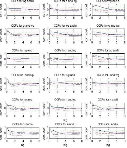
As an additional test of model fit, this appendix compares auto- and cross-correlation

func-tions generated from the model with collective bargaining and Finn (1998) calibrated for

Germany, with their empirical counterparts. The main emphasis in this subsection is on the

ACFs and CCFs of labor market variables. In particular, close attention is paid to cyclical

properties of public and private wage rates and hours. To establish 95% confidence intervals

for the theoretical ACFs and CCFs, as in Gregory and Smith (1991), the simulated time

series are used to obtain 1000 ACFs and CCFs. The mean ACFs and CCFs are computed by

averaging across simulations, as well as the corresponding standard error across simulations.

Those moments allow for the lower and upper bounds for the ACFs confidence intervals to

be estimated. The empirical ACFs and CCFs are then plotted, together with the theoretical

ones. If empirical ACFs lie within the confidence region, this means that the calibrated

model fits data well.

Empirical ACFs and CCFs were generated from a Vector Auto-Regressive (VAR) process of

order 1. Since ACFs and CCFs are robust to identifying restrictions (Canova (2007), Ch.7),

the VAR(1) was left unrestricted. The figures on the following pages display empirical ACFs

(solid line), together with the simulated average ACFs (dashed line) and the corresponding

stochastic error bounds (dotted lines). This is done for the union model first , and then for

the calibration using Finn’s (1998) framework.

The model with the public sector union calibrated for Germany outperforms Finn (1998),

especially in the prediction of the dynamic behavior of labor market variables. In terms

of capturing the autocorrelation structure of the variables, the union model fits data quite

well. One exception is the public sector wage: in data, it is highly autocorrelated, while the

model generates low persistence. A possible explanation could be that the public union puts

weight also on last year’s public sector wage level, i.e. _{the union bargains over the public}

wage increase rate, and not just the wage level. Public and total hours are also borderline

(25)

[image:25.612.114.522.129.608.2]

(26)

[image:26.612.112.523.127.619.2]

(27)

[image:27.612.114.522.130.607.2]

(28)

[image:28.612.114.521.129.608.2]

(29)

[image:29.612.112.523.127.620.2]

(30)

[image:30.612.114.522.130.608.2]

(31)

perfect positive contemporaneous correlation between public wages and hours, while in data,

it is negative. Overall, the model with public sector union calibrated for Germany captures

the dynamic co-movement of hours and wages with output, consumption and investment.

In addition, union model is able to address and match some new dimensions such as the

dynamic correlation of the two wage rates and the pair of hours worked.

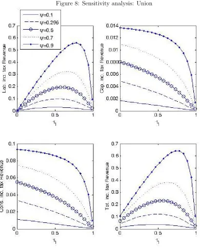
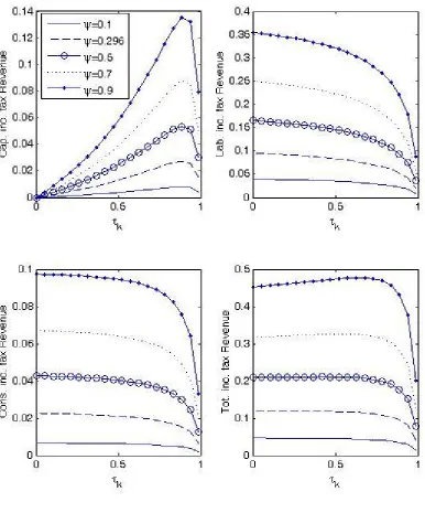
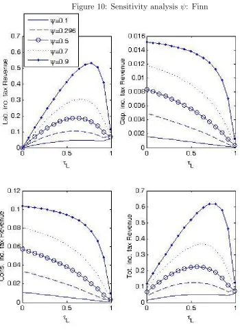
1.4 Sensitivity analysis

To evaluate the effect of structural parameters on the shape of the Laffer curves, this section

performs sensitivity analysis for different values of model parameters and how those affect

tax revenues. The two parameters of interest are the curvature parameter of household’s

Cobb-Douglas utility function α, as well as the weight on composite consumption, ψ.

In-terestingly, as α is allowed to vary, steady-state revenues are essentially unchanged. Even

an implausibly high value, α = 50, does not produce any difference in steady state tax

rev-enues. In both models considered in this paper, the preference parameter is not important

for steady-state fiscal policy effect. This result is not surprising in the literature, as Trabandt

and Uhlig (2010) obtain a very similar finding in their paper.1

In contrast, changes in the second parameter, ψ, yield significant differences. Both the

capital and labor tax Laffer curves, and the responses of the other tax bases to capital and

labor income tax rate are affected when ψ is allowed to vary.2 _{Higher values of} _ψ _{shift up}

the Laffer curve and make it steeper, without significant change in its peak. The difference

between Finn and the model with endogenous public employment becomes significant for

implausibly high values ofψ, i.e. ψ >0.5. (As explained in the calibration section,

parame-ter ψ = 0.296, describing household’s preference was calculated as the ratio of hours of work

out of total potential hours in the model.) Intuitively, a higher ψ corresponds to a lower

weight to leisure, (1−_ψ_{), in the household’s utility function. In other words, a higher} _ψ

1_Parameter_α_{is important for model dynamics, though.}

2_{Consumption tax Laffer curve proves to be very sensitive to}_ψ _{parameter. In the majority of the cases}

(32)

[image:32.612.99.496.118.568.2]

(33)

[image:33.612.103.493.80.573.2]

(34)

[image:34.612.98.484.120.585.2]

(35)

[image:35.612.102.452.77.558.2]

(36)

decreases the elasticity of private labor supply. Intuitively, when labor tax rate increases, or

equivalently, after tax private wage falls, private hours respond less, thus increasing labor

income tax revenue, as well as total tax revenue.

The effect of higher ψ on capital tax Laffer curve is similar to ψ’s effect on the labor tax

Laffer curve above. When τk _{is allowed to vary, a higher weight attached to consumption in}

household’s utility function, together with the optimality condition for the marginal rate of

substitution between consumption and hours require private higher capital stock to finance

private consumption. Therefore, a higher ψ shifts the capital tax Laffer curve upward as

well.

1.5 Measuring conditional welfare

In steady state

u(c, gc,1−_n_{) =} [(c+ωg

c₎ψ₍₁₋_n₎(1−ψ)

](1−α)₋

1

1−_α (186)

LetAandB denote two different regimes. The welfare gain,ζ, is the fraction of consumption

that is needed to complement household’s steady-state consumption in regimeB so that the

household is indifferent between the two regimes. Thus

[(cA₊_ωgc,A₎ψ₍₁₋_nA₎(1−ψ)

](1−α)₋

1

1−_α =

[((1 +ζ)cB₊_ωgc,B₎ψ₍₁₋_nB₎(1−ψ)

](1−α)₋

1

1−_α (187)

Multiply both sides by (1−_α_{) to obtain}

[(cA+ωgc,A)ψ(1−_nA₎(1−ψ)

](1−α)

−_{1 = [((1 +}_ζ₎_cB₊_ωgc,B₎ψ₍₁−_nB₎(1−ψ)

](1−α)

−_{1 (188)}

Cancel −_{1 terms at both sides to obtain}

[(cA+ωgc,A)ψ(1−_nA₎(1−ψ)

](1−α)

= [((1 +ζ)cB+ωgc,B)ψ(1−_nB₎(1−ψ)

](1−α)

(189)

Raise both sides to the power 1

1−α to obtain

(cA+ωgc,A)ψ(1−_nA₎(1−ψ)

= ((1 +ζ)cB+ωgc,B)ψ(1−_nB₎(1−ψ)

(190)

Divide throughout by (1−_nB₎(1−_ψ₎

to obtain

((1 +ζ)cB+ωgc,B)ψ = (cA+ωgc,A)ψ

1−_nA 1−_nB

(37)

Raise both sides to the power 1/ψ to obtain

(1 +ζ)cB₊_ωgc,B _{= (}_cA₊_ωgc,A₎

1−_nA 1−_nB

(1−_ψψ)

(191)

Move ωgc,B _{term to the right to obtain}

(1 +ζ)cB = (cA+ωgc,A)

1−_nA 1−_nB

(1−_ψψ)

−_ωgc,B ₍₁₉₂₎

Divide both sides by cB _{to obtain}

1 +ζ = 1

cB

(cA+ωgc,A)

1−_nA 1−_nB

(1−_ψψ)

−_ωgc,B

(193)

Thus

ζ = 1

cB

(cA+ωgc,A)

1−_nA 1−_nB

(1−_ψψ)

−_ωgc,B

−₁ ₍₁₉₄₎

Note that if ζ >0(<0), there is a welfare gain (loss) of moving from B toA. In this paper