Single Channel Source Separation Using Filterbank and 2D Sparse Matrix Factorization

Single Channel Source Separation Using Filterbank and

2D Sparse Matrix Factorization

Xiangying Lu1, Bin Gao1, Li Chin Khor1, Wai Lok Woo1, Satnam Dlay1, Wingkuen Ling2, Cheng S. Chin3

1_{School of Electrical and Electronic Engineering, Newcastle University, England, UK;} 2_{Faculty of Information Engineering,}

Guangdong University of Technology, Guangzhou, China; 3_{School of Marine Science and Technology, Newcastle University,} Eng-land, UK.

Email: bin.gao@ncl.ac.uk, w.l.woo@ncl.ac.uk

Received December 20th_{, 2012; revised January 23}rd_{, 2013; accepted January 31}st_{, 2013}

Copyright © 2013 Xiangying Lu etal. This is an open access article distributed under the Creative Commons Attribution License, which permits unrestricted use, distribution, and reproduction in any medium, provided the original work is properly cited.

ABSTRACT

We present a novel approach to solve the problem of single channel source separation (SCSS) based on filterbank tech- nique and sparse non-negative matrix two dimensional deconvolution (SNMF2D). The proposed approach does not require training information of the sources and therefore, it is highly suited for practicality of SCSS. The major problem of most existing SCSS algorithms lies in their inability to resolve the mixing ambiguity in the single channel observa- tion. Our proposed approach tackles this difficult problem by using filterbank which decomposes the mixed signal into sub-band domain. This will result the mixture in sub-band domain to be more separable. By incorporating SNMF2D algorithm, the spectral-temporal structure of the sources can be obtained more accurately. Real time test has been con- ducted and it is shown that the proposed method gives high quality source separation performance.

Keywords: Blind Source Separation; Non-Negative Matrix Factorization; Filterbank Analysis

1. Introduction

Blind source separation has gained a great deal of atten- tion in signal processing applications and these consist of medical signal analysis, telecommunications and speech recognition. There is an essential topic known as single channel source separation (SCSS) [1,2] which has not yet been enhanced enough to make its way out of laborato- ries. In recent years, new advances have been achieved in SCSS and this can be categorized into two main branches: supervised SCSS methods (e.g. model-based SCSS [3-6] techniques) and unsupervised SCSS methods (e.g. non- negative matrix factorization (NMF) [7] and computa- tional auditory scene analysis (CASA) [8]). In this paper, we proposed a novel unsupervised SCSS method based on non-negative matrix factorization approach.

NMF methods have been widely exploited in the field of SCSS, and especially being used in separating audio mixtures, e.g. extracting drums from polyphonic music [9] and automatic transcription of polyphonic music [10]. Families of parameterized NMF cost functions such as the Beta divergence [11] and Csiszar’s divergences [12] have been presented for the separation of audio signals

[13] and in general case, the least square distance [14] and the Kullback-Leibler (KL) divergence [15] are two main cost functions which have been widely employed in NMF. However, the problem where conventional NMF methods fail in SCSS is when two notes are played si- multaneously in which case they will be modeled as one component [7]. To overcome this limitation, the sparse non-negative matrix two dimensional deconvolu- tion (SNMF2D) [16] is derived to track the spectral fre- quencies of the sources that change over time.

SNMF2D. Once the sub-sources are obtained the k- means based clustering method is used to group these sub-sources into clusters where each cluster consist a set of sub-sources [17,18] which will be subsequently used for recovering the original sources. The proposed method concentrates on the idea of performance source separa- tion in the sub-band domain and avoids directly estimate- ing the sources using the mixture signal which contains too many mixing ambiguities between sources. In this way, we show that the proposed method can make a su- perior separation performance.

The paper is organized as follows: In Section 2, the pro- posed source separation framework is fully developed. In Section 3, experimental results are presented. The impact factors and a series of performance comparison are dis- cussed in Section 4. Finally, Section 5 concludes the paper.

2. Proposed Model

The single channel audio mixture x t

 

is given as:

 

1

 

2

 

x t s t s t (1) where denotes time index. The goal of SCSS is to estimate the two sources

1, 2, ,

t  T

 

1

s t and s t₂

 

when only the observation signal x t

 

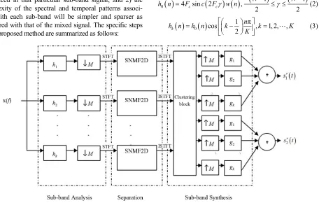
is available. The core procedure of the proposed method is shown in Figure 1. It consists of two main techniques-filterbank and SNMF2D. The benefits filterbank bring to SCSS are 1) the degree of mixing ambiguity from the original sources is reduced in that particular sub-band signal; and 2) the complexity of the spectral and temporal patterns associ- ated with each sub-band will be simpler and sparser as compared with that of the mixed signal. The specific steps of the proposed method are summarized as follows:

Step 1: Transform the mixture from time domain into sub-band domain using filterbank, and then down-sam- pling the signal for reducing the aliasing problem. Hence, instead of processing the mixed signal directly, the sub- band signals are utilized as the new set of observations.

Step 2: Convert the sub-band mixed signals into time- frequency (TF) domain by using STFT (Short-Time Fou- rier Transform) and then construct log-frequency magni- tude spectrogram, utilize SNMF2D to decompose the sub-band mixing TF mixtures into source related spectral and temporal patterns. The separated time domain sub- sources can be reconstructed by using the inverse STFT.

Step 3: Use the k-means clustering method to group the sub-sources into different clusters where each cluster consist a set of sub-sources correspond to one recovered source.

Step 4: Recover the time domain sources in the syn- thesis stage.

1) Pre-processingstage: Filterbank includes low-pass, band-pass, and high-pass filters which are served to iso- late different frequency components in a signal. The per- fect filterbank will be designed so that the output source is the same as the input source with no distortion through a time shift and amplitude scaling. Here, the down-sam- pling is served to reduce the aliasing [19-21] problem. In the sub-band analysis, the formulation of filterbank is given as follow:

 



   







0

1 1

4 sin 2 ,

2 2

c c

N N

h n  F c F w n      (2)

 

0

 

1 π

cos , 1, 2, ,

2 k

n

h n h n k k K

K

  

 _  _{ } 

 

[image:2.595.84.540.433.723.2]

   (3)

where the finite number of sub-bands is , is the length of window, the cut-off frequency is defined as

K N 1 4 c F K

 and w n

 

is the Hamming window given by

 

0.54 0.46cos 2nπ , 0,1, ,

w n n N

N

 

  _{ } 

   (4)

In this paper, the observations after filterbank proc- essing can be effectively down-sampled by an integer decimation factor r (down-sampling rate) in each sub-band. The down-sampled observation

D



,



x k p in the kth _{sub-band is generated by using} Equation (5), where r denotes the time index at the reduced sampling rate for some integer l , and

for avoiding [21] any aliasing distortion.



k1, 2,

K



K



,

p lD

D





  

1

, N k

n

x k p h n x p n











(5)

2) Separationstage: Once the new set of observations



,

x k p has been generated, the sub-band mixed signals are transformed to the time-frequency (TF) domain using STFT. We then group the spectrogram bins into 175 logarithmically spaced frequency bins in the range of 50 Hz to 8 kHz with 24 bins per octave, which corresponds to twice the resolution of the equal tempered musical scale to construct log-frequency [7] magnitude spectro- gram. Within the context of SCSS, the TF representation of the mixture in (1) is given by

.2 .2 .2

1 2

 

X S S (6)

where

 

1,2, ,

1,2, ,

,

s

i F

j T

X i j _  _ _

X 

 and

 

1,2, ,

1,2, , , s i d d F j T

S i j _  _ _

S _ are two-dimensional matrices

(row and column vector represents the time slots and frequencies, respectively). In this paper, we term the sources at each sub-band as the sub-sources. To estimate these sub-sources, we project all the sub-band mixed signals from (5) into the TF domain, in which can be denoted as:

12

2 _{s s}

x

k  k  k

C C C 22 ₍₇₎

2

x k

C and sd 2

k

C denotes TF representations of the kth _{sub-band mixture x k p}



_,



_{and d}th _{source, respec-} tively. The matrices we are interested to determine are

12

s k

C and s22

k

C which can be estimated using any non-negative matrix factorization algorithm. In our ap- proach, we favours the SNMF2D algorithm where the desirable matrices can be estimated as

12

,1 ,1

s

k k



Here, Wk d, denotes the dth column of Wk that corre-

sponds to the dth _{row of} ,

k d

H . In the case of two sources, we have d 

 

1, 2 . The reasons SNMF2D [19,20] are favoured over other conventional NMF methods are noted as follows: 1) The NMF does not model notes but rather unique events only. Thus, if two notes are always played simultaneously they will be modelled as one component; 2) The structure of a factor in H can be input into signature of the same factor in W and vice versa. Thus, this leads to ambiguity that can be resolved by forcing the structure on W through imposing sparseness on H. The two basic cost functions for optimizing Wk

and Hk d, are given by the Least Squares (LS) distance and Kullback-Leibler divergence (KLd) where is a sparseness parameter and f

 

H  H ₁:

LS:



, ,



2

 

,

1 2

SLS i j i j

i j

C 



V Λ f H (8)

KLd: ,

 

, , ,

, ,

log i j

SKL i j i j i j

i j i j

C 



V V V Λ f H

Λ



 (9)

In above, is the log-frequency magnitude spec- trogram, i j,

V

I J 



V is the data matrix of the sub-band

TF mixture and    

 





Λ W H where

 

2

, , ,

,

i d i d i d

i

  







W W W . The derivatives of (8) with

respect to W and H are given by:





 





, 2 , , , , , , , , 1 2 1 2 SLS i d

i j i j

i j i d

i j i j d j

j C f                             _{ }   





W

Y Λ H

W

Y Λ H

  (10)





 





 

, 2 , , , , , , , , , 1 2 1 2 SLS d j

i j i j

i j d j

i d i j i j

i d j

C f f                                    _{ }      





H

Y Λ H

H

H

W Y Λ

H 

 

(11)

Thus, by applying the standard gradient decent ap- proach, we have:

, ,

,

, ,

,

SLS

i d i d

i d

SLS

d j d j

d j C C                                   W H W W W H H H  (12) k        



C W H a n d 22

,2 ,2 s k k  k        



where W and H are positive learning rates which can be obtained by following the approach of Lee and

Seung [15], namely, , ,

,

i d i j d j

j       ,          _ 



W W Λ H 

 and

 

, , ,

, ,

d j i d i j

i d j

f                    _{ }  



H H

H W Λ

H



 _ 

. Thus, in matrix notation, by using the multiplicative learning rules, the SNMF2D algorithm are summarized in Table 1. In these tables, the superscript “ ” denotes vector transpose, “” is the element-wise product and at each iteration, denotes a matrix with the argument on the di- agonal. The column vectors of

T

 



diag



W will be factor-wise normalized to unit length.

After using mask, the sub-sources sa

k

c can be ob- tained:









1 1 2 2 1 1

s s x

k s s k k x k k c STFT c STFT       C C   mask mask _k (13)

where the masks are determined element-wise by:

2 2 , , , 1, if 0,otherwise a b a s s

s k _{i j} k _{i j}

k i j

 _{    }

 _{   }

  

C C

mask , (14)

3) Clusteringstage: Once the sub-sources are obtained by using inverse STFT, the k-means based clustering method is used to group these sub-sources into clusters according to the number of sources. In this case, the k-means method aims to separate 2 K observations (K is number of sub-bands) into two clusters (corresponding to two sources). After convergence, all sub-sources will be grouped into their respective clusters which are given

denoted as 2



2 2 2



2

1 , 2 , ,

s s s s

k  N

G c c   c and





2 2 2 2

2

1 , 2 , ,

s s s s

k 

G c c   c_N which contains N₁ and N2 number of sub-sources that belong to Source 1 and Source 2, respectively.

4) Synthesis stage: After up-sampling, the filterbank synthesis process is used to recombine all the sub- sources to form the estimated source signals. A series of expansions of the output can be reconstructed by using the time-shifted variants gk (synthesis filter) [19-21]. The process is expressed as follow:





 

 

0 0

0

1 , 1, 2, ,

1 π

cos 2 k

g h N n n N

n

g n g n k

K        _  _{ }     

 (15)

Finally, the recovered sources from each cluster can be estimated as

 

  



1 1 ˆ d K N s

d k k

k n

s t g n c t

 

n





  (16) where t t l M







denotes the time index at the restored sampling rate

 

M .

3. Experimental Results

The proposed monaural source separation algorithm is tested on recorded audio signals. Several experimental studies have been designed to investigate the efficacy of the proposed approach. All simulations and analysis are conducted using a PC with Intel Core 2 CPU 6600 @ 2.4 GHz and 2 GB RAM. For mixture generation, two sen- tences of the target speakers (male and female) “fcjf0” and “mcpm0”, were selected from TIMIT speech data-

Table 1. SNMF2D (LS and KL) algorithm. A) Initialize W and H are nonnegative randomly matrix

B) , ,

 

, 2 ,

i d i d i d

i

  







W W W

C)    

  



Λ W H

D)   f                     





W V H H H W Λ H    T

T (LS)  

f                         





V W Λ H H H W 1 H    T

T (KL)

E)    

  



Λ W H

F) diag diag       W W Λ                                  _   _            _ _  __      









V H W 1 V H W

H W 1 ΛH W

 

   

T T

T T (Least Square)

diag diag                                 _{    }     _{ }          _{ }        _{   } _      _{  }  









V

H W 1 1 H W

Λ

W W

V

1 H W 1 H W

Λ        T T T T

 _(Kullback

Liebler)

base and the others including flute, bass and drum music. All mixtures are sampled at 16 kHz sampling rate and the length of all test signals was chosen to be (40,000 sam- ples, approximately 2.5 s). The time-frequency represen- tation was computed by normalizing the time-domain signals to unit power and we computed the STFT using 1024 point Hanning window FFT with 50% overlap. The spectrogram bins are grouped into 175 logarithmically spaced frequency bins in the range of 50 Hz to 8 kHz with 24 bins per octave, which corresponds to twice the resolution of the equal tempered musical scale. As for the filterbank, the parameter corresponding to the total num- ber of filters is set as 4 and the length of the hamming window is defined equal to 128. As for SNMF2D pa- rameters, the convolutive components in frequency and

time were selected as and ,

respectively. The sparse regularization term is set to

K



0, , 4

 







0, ,10



6

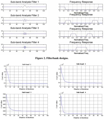
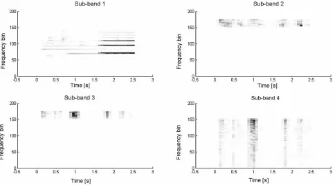
 . Figure 2 shows the design of four sub-bands. Using the filterbank is very useful and helpful for the

separation stage. This is because one of original sources may centralize its basic frequency information in a spe- cific sub-band such that the dominant source can be eas- ier extracted using source separation algorithms such as the SNMF2D. In the separation stage, the observed sig- nal in each sub-band is converted into the log-frequency spectrogram and decomposed by SNMF2D. The cost value of decomposing female speech mixed with bass music in each sub-band is shown in Figure 3. It is ob- served that the decomposition process converges to a low steady value after approximately 40 iterations for all sub-band mixtures by using the SNMF2D algorithm. Fig-

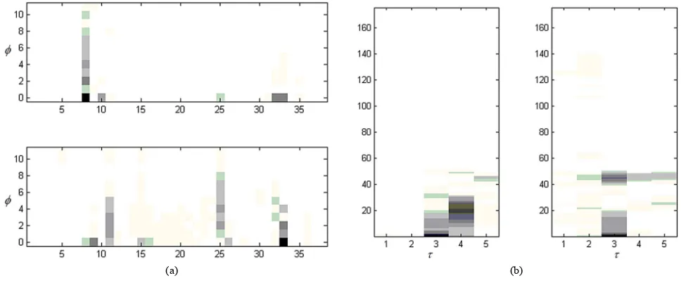
ure 4 shows an example of H and W as decomposed in

the fourth sub-band mixed signal. It is seen that the spec- tral bases and temporal codes of each source are distin- guishable so that each spectral basis can represent the frequency patterns of one sub-sources. The example of final separation results are shown in Figure 5.

[image:5.595.125.471.323.720.2]

The measure distortion between the original source

Figure 2. Filterbank designs.

[image:6.595.55.539.84.285.2]

(a) (b) Figure 4. (a) H (in fourth sub-band); (b) W (in fourth sub-band).

Figure 5. Original signals (blue) and recovered signals (red) using proposed method.

and the estimated one is computed by using the im- provement of signal-to-noise ratio (ISNR) [22] defined as:

 

 

 

 

 

 

2

10 2 10

10 log 10log

ˆ d

d

t t

d d d

t t

ISNR

s t s t 2

2

d

s t s t x t s t

 













(17) The ISNR is used as the quantitative measure of sepa- ration performance and the average ISNR will be tabu-

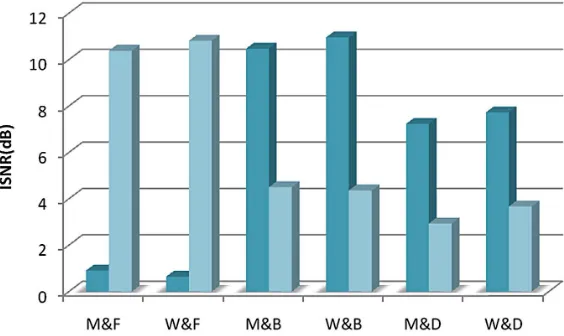
[image:6.595.54.546.152.553.2]

[image:7.595.157.439.553.721.2]

male speech, female speech, flute music, bass music and drum music. The separation of speech-bass music mix- ture is much better than those of other types of mixtures where the average ISNR has approached to 10 dB for recovered speech signal and 4 dB for recovered bass mu- sic.

Figure 6 summarizes the separation results of our pro- posed method. It is worth pointing out that because the frequency range of bass and drum music locate at very lower frequency region, the lower frequency bands are dominated with most energy from the bass or drum components through filterbank process. Hence, it is eas- ier to extract these lower frequency components by using the SNMF2D. Thus, Figure 6 shows the rela- tively better separation results when audio mixture contains bass or drum music. On the other hand, the frequency range of flute is very similar to speech sources (as indicated in Figure 9) and this particular mixture is very difficult to separate which explains the reason why the ISNR is relatively low. However, this performance is still substantially better than using the SNMF2D alone.

4. Discussion

4.1. Effects on Audio Mixtures Separation with/without Filterbank Preprocessing

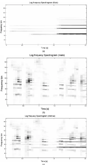
The benefits filterbank preprocessing bring to SCSS is that since a filtered signal bounded within a particular range of sub-band frequencies, the complexity of the spectral and temporal patterns associated with each sub- band signal will be simpler and sparser than that of the mixed signal. This effectively means that there is a rela- tively clear distinction of the spectral and temporal pat- terns between the dominating source and the less domi- nating one in the TF domain in each sub-band. This is shown in Figures 7 and 8.

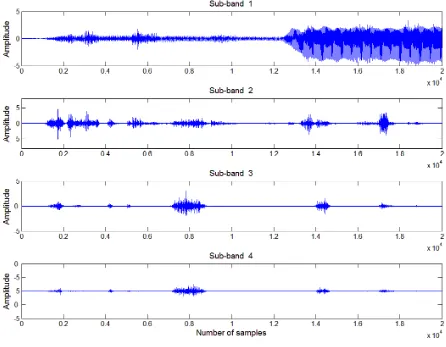
Figures 9 and 10 further show the time domain sub-

band signal. It is clearly visible that the mixing at the different sub-band is dominated either by Source 1 or Source 2. In this example, it can be seen that flute music dominates the 1st _{sub-band while male speech dominates} the 2nd_-4th_{sub-band. The final comparison results of audio} mixtures separation with/without filter-bank preprocess- ing are given in Figure 11.

4.2. Impact of Sparsity Regularization

In the separation stage, λ (sparse regularization), an es- sential parameter influences separation results. In Figure 7, we use an example-mixture of male speech and flute music for analyzing the impact of sparsity regularization. The separation results are concluded given different lev- els of sparse λbased on either LS or KLd cost functions. It is observed that the best ISNR has been found with the sparse factor λ = 6 by using the LS cost function and λ = 20 by using the KLd cost function. In addition, the LS cost function based decomposition reflects the local mi- nimum whereas the KLd based decomposition returns the global minimum. However, our results have shown that both LS and KLd methods give comparable performance as shown in Table 2.

In this section, we develop a test to compare the sepa- ration performance between the proposed method and SNMF2D SCSS method. Figure 11 shows that the ISNR results obtained using the proposed method which ren- ders considerable improvements over the SNMF2D SCSS method. An average improvement of 1.8 dB per source is obtained across all the different type of mixtures for proposed method when compared to SNMF2D SCSS method. The specific comparison results are summarized as follows: 1) for mixture of speech and flute music, the average improvement is about 3.4 dB; 2) for mixture of speech and bass music, the improvement is 1.5 dB; 3) for mixture of speech and drum music, the average improve- ment is approximately 0.2 dB.

(a)

(b)

(c)

[image:8.595.132.466.79.706.2]

[image:9.595.59.543.84.352.2] [image:9.595.72.527.367.718.2]

Figure 8. Log-frequency mixed spectrogram with filter-bank processing.

[image:10.595.74.520.86.433.2]

Figure 10. Time domain sub-band signals with filter-bank processing.

[image:10.595.61.287.451.589.2]

5. Conclusion

Figure 11. Overall comparison result.

Table 2. Separation results by using different sparse regu- larization.

λ LS KL

0 2.92 5.14

0.5 3.50 5.16 1.5 2.82 4.99

6 5.64 4.48

10 2.69 5.00

20 2.78 5.17

50 2.16 4.73

This paper has presented a novel framework of amalgam- mating filterbank technique with two-dimensional sparse non-negative matrix deconvolution (SNMF2D) for single channel source separation. Although proposed method and the SNMF2D SCSS method can extract sources from single channel mixture, the results obtained from our approach outperform that of using the SNMF2D. The strength of the proposed method: 1) it does not rely on training information so that it is more practical; 2) the degree of mixing ambiguity in each sub-band is less am- biguous than those in mixed signal; therefore the sub- band mixtures are simpler and sparser, and hence the spectral and temporal patterns can be efficiently extracted. Considerable improvements have been achieved in terms of ISNR by using our proposed method.

REFERENCES

[image:10.595.56.286.637.736.2]

[2] B. Gao, W. L. Woo and S. S. Dlay, “Single Channel Source Separation Using EMD-Subband Variable Regularized Sparse Features,” IEEE Transactions on Audio, Speech and Lang- uage Processing, Vol. 19, No. 4, 2011, pp. 961-976. doi:10.1109/TASL.2010.2072500

[3] M. H. Radfa and R. M. Dansereau, “Single-Channel Speech Separation Using Soft Mask Filtering,” IEEE Transac- tions on Audio, Speech and Language Processing, Vol. 15, No. 8, 2007, pp. 2299-2310.

[4] D. Ellis, “Model-Based Scene Analysis,” In: D. Wang and G. Brown, Eds. ComputationalAuditorySceneAna- lysis: Principles, Algorithms, and Applications, Wiley/ IEEE Press, New York, 2006.

[5] T. Kristjansson, H. Attias and J. Hershey, “Single Micro- Phone Source Separation Using High Resolution Signal Reconstruction,” Proceedings of the International Con-ference on Acoustics, Speech, and Signal Processing, Montreal, 17-21 May 2004, pp. 817-820.

[6] B. Gao, W. L. Woo and S. S. Dlay, “Adaptive Sparsity Non- Negative Matrix Factorization for Single Channel Source Separation,” IEEE Journal of Selected Topics in Signal Processing, Vol. 5, No. 5, 2011, pp. 1932-4553.

[7] G. J. Brown and M. Cooke, “Computational Auditory Scene Analysis,” Computer Speech and Language, Vol. 8, No. 4, 1994, pp. 297-336. doi:10.1006/csla.1994.1016

[8] M. Helén and T. Virtanen, “Separation of Drums from Polyphonic Music Using Nonnegative Matrix Factoriza- tion and Support Vector Machine,”13thEuropeanSignal ProcessingConference,Turkey, 6 September 2005. [9] P. Smaragdis and J. C. Brown, “Non-Negative Matrix

Factorization for Polyphonic Music Transcription,” IEEE WorkshoponApplicationsofSignalProcessingtoAudio andAcoustics (WASPAA), 19-22 October 2003, pp. 177- 180.

[10] R. Kompass, “A Generalized Divergence Measure for Non- negative Matrix Factorization,” ProceedingsoftheNeuro- informaticsWorkshop, Torun, September 2005.

[11] A. Cichocki, R. Zdunek, and S. I. Amari, “Csiszár’s di-vergences for non-negative matrix factorization: family of new algorithms,” Proceedings of the 6th International Conference on Independent Component Analysis and BlindSignalSeparation, Vol. 3889, Springer, Charleston,

2006, pp. 32-39. doi:10.1007/11679363_5

[12] P. D. O. Grady, “Sparse Separation of Under-Determined Speech Mixtures,” Ph.D. Thesis, National University of Ireland Maynooth, Kildare, 2007.

[13] D. Lee and H. Seung, “Learning the Parts of Objects by Nonnegative Matrix Factorisation,” Nature, Vol. 401, No. 6755, 1999, pp. 788-791. doi:10.1038/44565

[14] D. D. Lee and H. S. Seung, “Algorithms for Non-Nega- tive Matrix Factorization,” MIT Press, Cambridge, 2002, pp. 556-562.

[15] M. Mørup and M. N. Schmidt, “Sparse Non-Negative Ma- trix Factor 2-D Deconvolution for Automatic Transcrip- tion of Polyphonic Music,” Technical University of Denmark, Lyngby, 2006.

[16] A. Mertins, “Signal Analysis Wavelets, Filter Banks, Time- Frequency Transforms and Applications,” John Wiley & Sons, Hoboken, 1999, pp. 143-195.

[17] B. Gao, W. L. Woo and S. S. Dlay, “Variational Bayesian Re- gularized 2-D Nonnegative Matrix Factorization,” IEEE Transactions on Neural Networks and Learning Systems, Vol. 23, No. 5, 2012, pp. 703-716.

doi:10.1109/TNNLS.2012.2187925

[18] Md. K. I. Molla and K. Hirose, “Single-Mixture Audio Source Separation by Subspace Decomposition of Hilbert Spectrum,” The IEEE Transactions on Audio, Speech and Language Processing, Vol. 15, No. 3, 2007, pp. 893-900. [19] J. Taghia and M. Ali Doostari, “Subband-Based Single-

Channel Source Separation of Instantaneous Audio Mix- tures,” World Applied Sciences Journal, Vol. 6, No. 6, 2009, pp. 784-792.

[20] K. Kokkinakis and P. C. Loiziu, “Subband-Based Blind Signal Processing for Source Separation in Convolutive Mixtures of Speech,” IEEEInternationalConference on Acoustic, SpeechandSignalProcessing, Honolulu, 15-20 April 2007, pp. 917-920.

[21] P. P. Vaidyanathan, “Multirate Systems and Filter Banks,” Prentice-Hall, Englewood Cliffs, 1993.